1.1 Notes on Assumption (2.) 1.1.1 The unconditional mean of the - PDF document

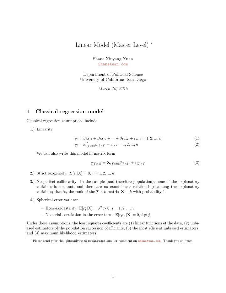
Linear Model (Master Level) ∗ Shane Xinyang Xuan ShaneXuan.com Department of Political Science University of California, San Diego March 16, 2018 1 Classical regression model Classical regression assumptions include 1.) Linearity y i = β 1 x i 1 + β 2 x i 2 + ... + β k x ik + ε i , i = 1 , 2 , ..., n (1) y i = x i ′ (1 × k ) β ( k × 1) + ε i , i = 1 , 2 , ..., n (2) We can also write this model in matrix form y ( T × 1) = X ( T × k ) β ( k × 1) + ε ( T × 1) (3) 2.) Strict exogeneity: E [ ε i | X ] = 0 , i = 1 , 2 , ..., n 3.) No perfect collinearity: In the sample (and therefore population), none of the explanatory variables is constant, and there are no exact linear relationships among the explanatory variables; that is, the rank of the T × k matrix X is k with probability 1 4.) Spherical error variance: i | X ] = σ 2 > 0 , i = 1 , 2 , ..., n – Homoskedasticity: E [ ε 2 – No serial correlation in the error term: E [ ε i ε j | X ] = 0 , i � = j Under these assumptions, the least squares coefficients are (1) linear functions of the data, (2) unbi- ased estimators of the population regression coefficients, (3) the most efficient unbiased estimators, and (4) maximum likelihood estimators. ∗ Please send your thoughts/advice to xxuan@ucsd.edu , or comment on ShaneXuan.com . Thank you so much. 1

1.1 Notes on Assumption (2.) 1.1.1 The unconditional mean of the error term is zero The unconditional mean of the error term is zero. The law of total expectations states that E [ E ( y | x )] = E [ y ] (4) Since E [ ε i | X ] = 0 , we know that E [ ε i ] = E [ E ( ε i | X )] = 0 (5) 1.1.2 The regressors are orthogonal to the error term We first apply the law of iterated expectations: E [ x i ε i ] = E [ E ( x i ε i | x i )] (6) It follows that E [ x i ε i ] = E [ x i E ( ε i | x i )] = 0 Hence, we have shown that E [ x i ε i ] = 0 for every observation. 1.2 Notes on Assumption (4.) We can write Assumption (4.) in a more compact way: E [ εε ′ | X ] = σ 2 I T (7) ≡ var( ε | X ) (8) For example, the ( i, j ) element of the T × T matrix εε ′ is ε i ε j , and E [ ε i ε j ] = 0 because the ( i, j ) element is on the off-diagonal of matrix εε ′ . In sum, Equation (8) is a compact way that assumes both homoskedasticity, and no serial correlation in the error term. This assumption will be relaxed in certain circumstances. 2

2 Finite sample properties of b Unbiased Under Assumptions (1.)–(3.), E [ b | X ] = β Proof. To prove this property, we just need to show E [ b − β | X ] = 0. Note that E [ b − β | X ] = E [( X ′ X ) − 1 X ′ ε | X ] = ( X ′ X ) − 1 X ′ E [ ε | X ] = 0 � Variance Under Assumptions (1.)–(4.), var( b | X ) = σ 2 ( X ′ X ) − 1 Proof. var( b | X ) = E [( b − β ) 2 | X ] (9) = E [( b − β )( b − β ) ′ | X ] (10) A ′ = ( X ′ X ) − 1 X ′ = E [ Aεε ′ A ′ | X ] , (11) = A E [ εε ′ | X ] A ′ (12) = σ 2 AA ′ (13) = σ 2 ( X ′ X ) − 1 X ′ X ( X ′ X ) − 1 (14) � �� � I k = σ 2 ( X ′ X ) − 1 (15) � 3