1.1 Dynamics of a Cumulus topped Boundary Layer: an analysis of LES - PDF document
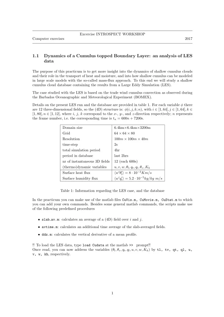
Excercise INTROSPECT WORKSHOP Computer exercises 2017 1.1 Dynamics of a Cumulus topped Boundary Layer: an analysis of LES data The purpose of this practicum is to get more insight into the dynamics of shallow cumulus clouds and their role in
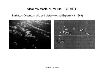
Excercise INTROSPECT WORKSHOP Computer exercises 2017 1.1 Dynamics of a Cumulus topped Boundary Layer: an analysis of LES data The purpose of this practicum is to get more insight into the dynamics of shallow cumulus clouds and their role in the transport of heat and moisture, and into how shallow cumulus can be modeled in large scale models with the so-called mass-flux approach. To this end we will study a shallow cumulus cloud database containing the results from a Large Eddy Simulation (LES). The case studied with the LES is based on the trade wind cumulus convection as observed during the Barbados Oceanographic and Meteorological Experiment (BOMEX). Details on the present LES run and the database are provided in table 1. For each variable φ there are 12 three-dimensional fields, so the (4D) structure is: φ ( i, j, k ; n ), with i ∈ [1 , 64] , j ∈ [1 , 64] , k ∈ [1 , 80] , n ∈ [1 , 12], where i , j , k correspond to the x -, y -, and z -direction respectively; n represents the frame number, i.e. the corresponding time is t n = 600 n + 7200s. Domain size 6.4km × 6.4km × 3200m Grid 64 × 64 × 80 Resolution 100 m × 100 m × 40 m time-step 2s total simulation period 4hr period in database last 2hrs nr of instantaneous 3D fields 12 (each 600s) (thermo)dynamic variables u, v, w, θ l , q t , q l , θ v , K h l � = 8 · 10 − 3 Km/s Surface heat flux � w ′ θ ′ t � = 5 . 2 · 10 − 5 kg/kg m/s Surface humidity flux � w ′ q ′ Table 1: Information regarding the LES case, and the database In the practicum you can make use of the matlab files CuVis.m, CuMovie.m, CuStat.m to which you can add your own commands. Besides some general matlab commands, the scripts make use of the following predefined procedures • slab av.m : calculates an average of a (4D) field over i and j . • avtime.m : calculates an additional time average of the slab-averaged fields. • ddz.m : calculates the vertical derivative of a mean profile. !! To load the LES data, type load Cudata at the matlab >> prompt!! Once read, you can now address the variables ( θ l , θ v , q t , q l , u, v, w, K h ) by tl, tv, qt, ql, u, v, w, kh , respectively. 1
3D Visualization of Clouds a. Run CuVis . The liquid water data q l are now processed and a snapshot of a 3D cloud field becomes visible. You can rotate and zoom the image to have a better look at the data. b. Increase the threshold in the isosurface routine. What effect does it have on small and big clouds? c. Start CuMovie : this will generate an animation of the evolution of the cloud field over the last two hours (12 frames). Mean Profiles d. Start CuStat . As an example the code will calculate the slab average of liquid water: 1 � q l ( k ; n ) = q l ( i, j, k ; n ) N x N y ij and plot the instantaneous profiles. Next it will additionally average these profiles in time and plot the result, i.e. � q l � = 1 � q l ( k ; n ) N t n What is the typical value for the average liquid water content in the cloud layer? e. Add your commands to the file CuStat.m to study the profiles of the thermodynamic variables q t , θ l , and θ v . Identify the cloud-layer, the sub-cloud layer and the free troposphere. Fluxes Remove the comment symbols in the matlab file below ’Fluxes’. The code fragment calculates the both the resolved and subgrid fluxes of a variable. f. Average the fluxes additionaly over time and plot � w ′ q ′ t � , � w ′ θ ′ l � . Conditional Sampling and Cloud Averages Here we will determine the cloud-averaged values of various quantities. In this way we also get the cloud mass-flux, and therefore insight into the vertical transport by cumulus clouds. Conditional averages can be easily derived from the data by defining an ’indicator’ field that mark the cloudy points � 0 if q l ( i, j, k ; n ) = 0 c ( i, j, k ; n ) = 1 if q l ( i, j, k ; n ) > 0 Then the (average) cloud fraction at level k is given by 1 � σ = c ( i, j, k ; n ) = � c � N x N y N t ijn The average cloud mass-flux at level k is given by 1 � M = c ( i, j, k ; n ) w ( i, j, k ; n ) = � c w � N x N y N t ijn The ’cloud average’ value of an arbitrary variable φ can be determined by � ijn c ( i, j, k ; n ) φ ( i, j, k ; n ) = � c φ � φ c = � ijn c ( i, j, k ; n ) � c � g. Remove the comment symbols below ’Conditional sampling’. In matlab it is very easy to construct the indicator field by the command: c = ql > 0 . Next the code fragment calculates 2
and plots the cloud fraction profile. Add your commands to the code to calculate and plot the mass-flux profile. h. Plot profiles of the cloud averaged vertical velocity w c . i. Plot profiles of the cloud averaged liquid water q c l , total water q c t , and the cloud values θ c l , θ c v . Compare with the mean profiles. How big is the θ v -excess (difference between the cloud value and mean value, θ c v − � θ v � )? Compare to the θ l -excess. Discuss the differences between these excesses. Mass-flux Model The ’top-hat’ approximation for cumulus clouds enables one to model fluxes in the following man- ner: � w ′ φ ′ � = M ( φ c − φ ) (1) j. Check how well equation (1) approximates the fluxes of q t and θ l , by plotting the left-hand side and the right-hand side of the equation in the same plot. The fractional entrainment rate ǫ can be diagnosed from the q t profile by computing − dq c t dz ǫ = q c t − q t k. Plot the computed fractional entrainment rate ǫ profile. 3
1.2 Entraining parcels In exercise 1.2, we’ve experimented with dry and moist parcel ascent for parcels that don’t mix with their surroundings. However, when a parcel rises, there will inevitably be some exchange with the environment. Lateral mixing concerns the mixing of environmental air into the parcel (entrainment) as well the mixing of air from the parcel into the environment (detrainment) as the parcel rises. For steady state, the governing equations of a parcel can be written as ∂M c = E − D, (2) ∂z ∂M c φ c = Eφ e − Dφ c . (3) ∂z Here, M c is the mass flux, E and D represent the entrainment and detrainment, respectively, and φ = { θ l , q t } . We assume E and D to be related to the mass flux, which leads to the following parameterization: E = ǫM c , D = δM c , with ǫ and δ entrainment and detrainment rates, which we will assume to be constant. a. (@home) Show that the profiles of q t and θ l can be written in the form ∂φ ∂z = − ǫ ( φ c − φ e ) , φ = { θ l , q t } . (4) We will now study parcel ascent using mean profiles based on the BOMEX experiment. These profiles are defined in the Bomexprofs.m function. A parcel is given an excess ∆ q t and ∆ θ l at the surface to initialize ascent, so that q t,c ( z 0 ) = q t,e ( z 0 ) + ∆ q t , (5) θ l,c ( z 0 ) = θ l,e ( z 0 ) + ∆ θ l . (6) quantity value unit p 0 10 5 Pa θ l,e ( z 0 ) 298.7 K 17 · 10 − 3 kg (kg) − 1 q t,e ( z 0 ) ∆ θ l 0.1 K 0 . 3 · 10 − 3 kg (kg) − 1 ∆ q t 2 · 10 − 3 m − 1 ǫ JK − 1 (kg) − 1 R d 287.04 JK − 1 (kg) − 1 R v 461.5 kg m − 3 ρ 1.2 JK − 1 (kg) − 1 c p 1004 JK − 1 2 . 5 · 10 6 L v Table 2: Physical constants and parameter settings. b. Open start-parcels.m , and plot the profiles of environmental versus parcel θ l , q t , θ v and q l for undiluted ascent (i.e. ǫ = 0 m − 1 ). At which height does a cloud form? How far does the parcel rise until it becomes neutrally buoyant? c. Next, implement lateral entrainment by modifying the equations for θ l and q t , using equation (4). Use a value of ǫ = 2 · 10 − 3 m − 1 . Plot the entrained profiles in the same figures used in 1.2.b. At which heights are cloud base and cloud top located? 4
d. Use different values of ǫ . How does this affect parcel ascent? Explain why. Though the parcel is no longer buoyant when it has the same virtual potential temperature as the environment, it can continue to rise a bit further due to its vertical velocity. This process is called overshooting. The vertical velocity equation can be written as: 1 ∂w 2 c + 0 . 6 g θ v,c − θ v,e c ∂z = − ǫw 2 . (7) 2 θ v,e e. (@home) Which process does the second RHS term represent, and why its strength is reduced to 60%? f. Plot the vertical velocity profile. At which height does the velocity become zero? Does this coincide with the cloud top height found in 1.2.c? 5
Recommend
More recommend
Explore More Topics
Stay informed with curated content and fresh updates.

