xtdpdml for Estimating Dynamic Panel Models Enrique Moral-Benito - PowerPoint PPT Presentation
xtdpdml for Estimating Dynamic Panel Models Enrique Moral-Benito Richard Williams Paul Allison Banco de Espa na University of Pennsylvania University of Notre Dame Reuni on Espa nola de Usuarios de Stata
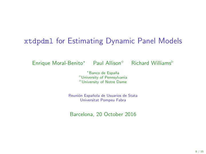
xtdpdml for Estimating Dynamic Panel Models Enrique Moral-Benito ⋆ Richard Williams ⊲ Paul Allison ⋄ ⋆ Banco de Espa˜ na ⋄ University of Pennsylvania ⊲ University of Notre Dame Reuni´ on Espa˜ nola de Usuarios de Stata Universitat Pompeu Fabra Barcelona, 20 October 2016 0 / 15
Motivation Source: Linnemer and Visser (2016) The Most Cited Articles from the Top-5 Journals (1991-2015). 1 / 15
A gentle reminder The model y it = λy it − 1 + βx it + α i + v it (1) v it | y t − 1 , x t � � E i , α i = 0 (2) i The Arellano-Bond approach ( T = 3 ) E ( y i 0 ∆ v i 2 ) = 0 (3a) E ( x i 1 ∆ v i 2 ) = 0 (3b) E ( y i 0 ∆ v i 3 ) = 0 (3c) E ( y i 1 ∆ v i 3 ) = 0 (3d) E ( x i 1 ∆ v i 3 ) = 0 (3e) E ( x i 2 ∆ v i 3 ) = 0 (3f) 2 / 15
In a nutshell Arellano-Bond may be biased in finite samples (moderate N , small T ) when instruments are weak (Alonso-Borrego and Arellano 1999). Several GMM alternatives have been proposed to address this concern (see Hansen et al. 1996; Alonso-Borrego and Arellano 1999). A practical limitation of these alternatives is that their implementation requires certain programming capabilities. The most popular alternative is thus the so-called system-GMM estimator by Arellano and Bover (1995) that can be easily implemented in Stata: System-GMM requires the mean stationarity assumption for consistency. 3 / 15
In a nutshell Arellano-Bond may be biased in finite samples (moderate N , small T ) when instruments are weak (Alonso-Borrego and Arellano 1999). Several GMM alternatives have been proposed to address this concern (see Hansen et al. 1996; Alonso-Borrego and Arellano 1999). A practical limitation of these alternatives is that their implementation requires certain programming capabilities. The most popular alternative is thus the so-called system-GMM estimator by Arellano and Bover (1995) that can be easily implemented in Stata: System-GMM requires the mean stationarity assumption for consistency. We consider a likelihood-based estimator that alleviates these biases based on the same identifying assumptions as Arellano-Bond. We introduce the Stata command xtdpdml that implements this estimator. It is already available from the Boston College Statistical Software Components (SSC) archive: ssc install xtdpdml See Williams, Allison and Moral-Benito (2016) available at http://www3.nd.edu/ ∼ rwilliam/dynamic/. 3 / 15
Roadmap The likelihood function . Monte Carlo evidence. Empirical illustration. The xtdpdml command. 3 / 15
The model in matrix form In addition to the T equations given by (1), we complete the model with an equation for y i 0 as well as T additional reduced-form equations for x : = (4) y i 0 v i 0 = (5) x i 1 ξ i 1 . . . x iT = ξ iT (6) In order to rewrite the system of equations given by (1) and (4)-(6) in matrix form, we define the following vectors of observed data ( R i ) and disturbances ( U i ): = ( y i 1 , ..., y iT , y i 0 , x i 1 , ...x iT ) ′ (7) R i = ( α i , v i 1 , ..., v iT , v i 0 , ξ i 1 , ...ξ iT ) ′ (8) U i So that: BR i = DU i (9) 4 / 15
The likelihood function Under normality, the joint distribution of R i is: � 0 , B − 1 D Σ D ′ B ′− 1 � R i ∼ N (10) with resulting log-likelihood: N L ∝ − N − 1 B − 1 D Σ D ′ B ′− 1 � − 1 R i � � B − 1 D Σ D ′ B ′− 1 � � 2 log det R ′ (11) i 2 i =1 The maximizer of L is asymptotically equivalent to the Arellano and Bond (1991) GMM estimator regardless of non-normality. The parameters to be estimated are place in the matrices B , D , and Σ . 5 / 15
Roadmap The likelihood function. Monte Carlo evidence . Empirical illustration. The xtdpdml command. 5 / 15
Simulation experiment We explore the finite sample behavior of our ML estimator compared to Arellano-Bond. We consider the simulation setting in Bun and Kiviet (2006). The data for the dependent variable y and the explanatory variable x are generated according to: y it = λy it − 1 + βx it + α i + v it (12) x it = ρx it − 1 + φy it − 1 + πα i + ξ it (13) where v it , ξ it , and α i are generated as v it ∼ i.i.d. (0 , 1) , ξ it ∼ i.i.d. (0 , 6 . 58) , and α i ∼ i.i.d. (0 , 2 . 96) . The parameter φ in (13) captures the feedback from the lagged dependent variable to the regressor. With respect to the parameter values, we fix λ = 0 . 75 , β = 0 . 25 , ρ = 0 . 5 , φ = − 0 . 17 , and π = 0 . 67 . This configuration allows for fixed effects correlated with the regressor as well as feedback from y to x . 6 / 15
Simulation results (I) Table: Simulation results. Bias λ Bias β iqr λ iqr β AB ML AB ML AB ML AB ML Sample size (1) (2) (3) (4) (5) (6) (7) (8) N = 100 , T = 4 -0.207 -0.007 -0.079 -0.005 0.359 0.238 0.158 0.120 N = 200 , T = 4 -0.150 -0.009 -0.061 -0.003 0.307 0.187 0.141 0.092 N = 500 , T = 4 -0.074 0.005 -0.030 -0.002 0.230 0.153 0.100 0.079 N = 1000 , T = 4 -0.041 0.012 -0.018 0.005 0.178 0.147 0.075 0.063 N = 5000 , T = 4 -0.006 0.001 -0.002 0.001 0.078 0.062 0.033 0.028 N = 100 , T = 8 -0.068 0.011 -0.012 0.005 0.078 0.089 0.034 0.042 N = 100 , T = 12 -0.040 -0.001 -0.004 0.000 0.046 0.046 0.019 0.023 N = 5000 , T = 12 -0.001 0.000 0.000 0.000 0.008 0.006 0.003 0.003 Notes. AB refers to the Arellano and Bond (1991) GMM estimator; Bias refer to the median estimation errors ˆ λ − λ and ˆ β − β ; iqr is the 75 th -25 th interquartile range; results are based on 1,000 replications. We use the xtdpdml Stata command for ML and the xtdpd Stata command for AB. 7 / 15
Simulation results (II) Table: Simulation results under unbalanced panels. Bias λ Bias β iqr λ iqr β AB ML AB ML AB ML AB ML Unbalacedness (1) (2) (3) (4) (5) (6) (7) (8) PANEL A: N = 200 , T = 4 1% -0.171 -0.005 -0.063 0.006 0.336 0.212 0.134 0.099 5% -0.218 -0.004 -0.082 0.000 0.381 0.212 0.153 0.091 10% -0.268 0.005 -0.111 0.003 0.381 0.222 0.154 0.100 PANEL B: N = 500 , T = 4 1% -0.090 -0.003 -0.035 -0.003 0.235 0.160 0.100 0.071 5% -0.122 0.009 -0.051 0.005 0.282 0.155 0.114 0.070 10% -0.163 0.016 -0.065 0.005 0.307 0.175 0.125 0.074 PANEL C: N = 200 , T = 8 1% -0.049 0.004 -0.009 0.004 0.067 0.067 0.027 0.029 5% -0.072 0.015 -0.015 0.010 0.081 0.083 0.032 0.034 10% -0.104 0.020 -0.027 0.014 0.099 0.087 0.042 0.036 PANEL D: N = 500 , T = 8 1% -0.021 0.006 -0.004 0.003 0.043 0.037 0.018 0.017 5% -0.035 0.014 -0.008 0.007 0.053 0.043 0.021 0.018 10% -0.054 0.022 -0.015 0.011 0.063 0.048 0.026 0.019 Notes. AB refers to the Arellano and Bond (1991) GMM estimator; Bias refer to the median estimation errors ˆ λ − λ and ˆ β − β ; iqr is the 75 th -25 th interquartile range; results are based on 1,000 replications. We use the xtdpdml Stata command for ML and the xtdpd Stata command for AB. 8 / 15
Roadmap The likelihood function. Monte Carlo evidence. Empirical illustration . The xtdpdml command. 8 / 15
Empirical illustration (I) The growth regressions literature is based on panel data methods accounting for country-specific effects and reverse causality between economic growth and potential growth determinants. The influential paper by Levine et al. (2000) found a positive effect of financial development on economic growth using the Arellano-Bond estimator. They estimate the following model: y it = λy it − 1 + βFD it + γw it + α i + v it (14) where y it refers to the log of real per capita GDP in country i and lustrum t , FD it refers to financial development, and w it refers to a set of control variables. [Details]. Following Levine et al. (2000) we assume that both FD it and the control variables w it are predetermined so that feedback from GDP to financial development and other macroeconomic conditions is allowed: v it | y t − 1 , w t i , FD t � � E i , α i = 0 ( t = 1 , ..., T )( i = 1 , ..., N ) (15) i 9 / 15
Recommend
More recommend
Explore More Topics
Stay informed with curated content and fresh updates.










![COMMUNICATING [with empathy] @ DY DYNAMIC JILL JILL @ DY DYNAMIC JILL TENSION IS INEVITABLE @](https://c.sambuz.com/548934/communicating-s.webp)
