Windowing Overview Windowing Relevance In practice, we cannot - PowerPoint PPT Presentation

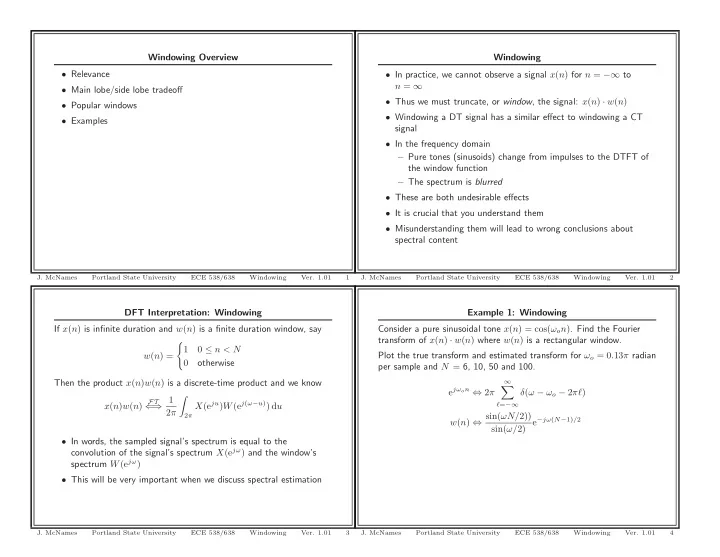
Windowing Overview Windowing • Relevance • In practice, we cannot observe a signal x ( n ) for n = −∞ to n = ∞ • Main lobe/side lobe tradeoff • Thus we must truncate, or window , the signal: x ( n ) · w ( n ) • Popular windows • Windowing a DT signal has a similar effect to windowing a CT • Examples signal • In the frequency domain – Pure tones (sinusoids) change from impulses to the DTFT of the window function – The spectrum is blurred • These are both undesirable effects • It is crucial that you understand them • Misunderstanding them will lead to wrong conclusions about spectral content J. McNames Portland State University ECE 538/638 Windowing Ver. 1.01 1 J. McNames Portland State University ECE 538/638 Windowing Ver. 1.01 2 DFT Interpretation: Windowing Example 1: Windowing If x ( n ) is infinite duration and w ( n ) is a finite duration window, say Consider a pure sinusoidal tone x ( n ) = cos( ω o n ) . Find the Fourier transform of x ( n ) · w ( n ) where w ( n ) is a rectangular window. � 1 0 ≤ n < N w ( n ) = Plot the true transform and estimated transform for ω o = 0 . 13 π radian 0 otherwise per sample and N = 6, 10, 50 and 100. Then the product x ( n ) w ( n ) is a discrete-time product and we know ∞ e jω o n ⇔ 2 π � δ ( ω − ω o − 2 πℓ ) ⇒ 1 � FT X (e ju ) W (e j ( ω − u ) ) d u ℓ = −∞ x ( n ) w ( n ) ⇐ 2 π 2 π w ( n ) ⇔ sin( ωN/ 2)) sin( ω/ 2) e − jω ( N − 1) / 2 • In words, the sampled signal’s spectrum is equal to the convolution of the signal’s spectrum X (e jω ) and the window’s spectrum W (e jω ) • This will be very important when we discuss spectral estimation J. McNames Portland State University ECE 538/638 Windowing Ver. 1.01 3 J. McNames Portland State University ECE 538/638 Windowing Ver. 1.01 4

Example 1: N = 6 Example 1: N = 10 Windowed Cosine N=6 Windowed Cosine N=10 1 1 x(n) w(n) x(n) w(n) 0 0 −1 −1 0 20 40 60 80 100 0 20 40 60 80 100 Time (n) Time (n) X(e j ω ) * W(e j ω ) X(e j ω ) * W(e j ω ) 5 20 0 0 −3 −2 −1 0 1 2 3 −3 −2 −1 0 1 2 3 Frequency (rad/sample) Frequency (rad/sample) X(e j ω ) * W(e j ω ) X(e j ω ) * W(e j ω ) 0 10 0 10 −3 −2 −1 0 1 2 3 −3 −2 −1 0 1 2 3 Frequency (rad/sample) Frequency (rad/sample) J. McNames Portland State University ECE 538/638 Windowing Ver. 1.01 5 J. McNames Portland State University ECE 538/638 Windowing Ver. 1.01 6 Example 1: N = 50 Example 1: N = 100 Windowed Cosine N=50 Windowed Cosine N=100 1 1 x(n) w(n) x(n) w(n) 0 0 −1 −1 0 20 40 60 80 100 0 20 40 60 80 100 Time (n) Time (n) X(e j ω ) * W(e j ω ) X(e j ω ) * W(e j ω ) 2000 500 1000 0 0 −3 −2 −1 0 1 2 3 −3 −2 −1 0 1 2 3 Frequency (rad/sample) Frequency (rad/sample) X(e j ω ) * W(e j ω ) X(e j ω ) * W(e j ω ) 2 10 0 10 −3 −2 −1 0 1 2 3 −3 −2 −1 0 1 2 3 Frequency (rad/sample) Frequency (rad/sample) J. McNames Portland State University ECE 538/638 Windowing Ver. 1.01 7 J. McNames Portland State University ECE 538/638 Windowing Ver. 1.01 8

Example 1: MATLAB Code Example 1: MATLAB Code Continued N = [6 10 50 100]; n = -10:(max(N)+10); subplot(3,1,2); nz = 2^12; % Number of zeros for padding h = plot(w,Rx,’r’,’LineWidth’,0.6); k = (1:nz/2+1); % Frequency indices xlim([-pi pi]); w = 2*pi*(k-1)/nz; % Frequencies (rads/sample) ylim([0 max(Rx)*1.05]); w = [-fliplr(w) w(2:end)]; % Include negative frequencies hold on; wo = 0.13*pi; % Frequency of the sinusoid h = plot(wo*[1 -1;1 -1],[0 0;1 1]*max(Rx),’g’); hold off; for cnt = 1:length(N), xlabel(’Frequency (rad/sample)’); wn = (n>=0 & n<N(cnt)); ylabel(’X(e^{j\omega}) * W(e^{j\omega})’); x = cos(wo*n).*wn; box off; X = fft(x,nz); subplot(3,1,3); Rx = abs(X(k)).^2; h = semilogy(w,Rx,’r’,’LineWidth’,0.6); Rx = [fliplr(Rx) Rx(2:end)]; % Include negative frequencies xlim([-pi pi]); figure; ylim(max(Rx)*[0.001 1.05]); subplot(3,1,1); hold on; h = stem(n,x,’filled’); h = plot(wo*[1 -1;1 -1],[0.001 0.001;1 1]*max(Rx),’g’); set(h(1),’MarkerFaceColor’,’b’); hold off; set(h(1),’MarkerSize’,2); xlabel(’Frequency (rad/sample)’); xlim([min(n) max(n)]); ylabel(’X(e^{j\omega}) * W(e^{j\omega})’); ylim([-1.05 1.05]); box off; xlabel(’Time (n)’); end; ylabel(’x(n) w(n)’); title(sprintf(’Windowed Cosine N=%d’,N(cnt))); box off; J. McNames Portland State University ECE 538/638 Windowing Ver. 1.01 9 J. McNames Portland State University ECE 538/638 Windowing Ver. 1.01 10 Windowing Example 2: Fixed Windows � π ⇒ 1 Plot various fixed windows and their Fourier transform. Center the FT X (e ju ) W (e j ( ω − u ) ) d u x ( n ) w ( n ) ⇐ windows so that they have even symmetry and length N = 25 samples. 2 π − π • Windowing in the time domain is equivalent to convolution in the frequency domain • Would like window to be as close as a Dirac impulse as possible • Length of window is constrained to N samples • Key tradeoff: main lobe width an amplitude of side lobes – Both can cause bias in the frequency domain • There are many windows to chose from • Rectangular window has smallest main lobe, but largest side lobes • Two types of windows – Fixed: defined only by the duration of the window, N – Parametric: have parameters that control the tradeoff between main lobe width and side lobe amplitude J. McNames Portland State University ECE 538/638 Windowing Ver. 1.01 11 J. McNames Portland State University ECE 538/638 Windowing Ver. 1.01 12

Example 2: Rectangular Example 2: Triangular Rectangular Length:25 Triangular Length:25 1 Window Window 1 0.5 0 0 −10 −5 0 5 10 −10 −5 0 5 10 20 20 W(e j ω ) W(e j ω ) 10 10 0 0 −3 −2 −1 0 1 2 3 −3 −2 −1 0 1 2 3 0 0 10 10 |W(e j ω )| |W(e j ω )| −3 −2 −1 0 1 2 3 −3 −2 −1 0 1 2 3 ω (rad/sec) ω (rad/sec) J. McNames Portland State University ECE 538/638 Windowing Ver. 1.01 13 J. McNames Portland State University ECE 538/638 Windowing Ver. 1.01 14 Example 2: Hamming Example 2: Hanning Hamming Length:25 Hanning Length:25 Window Window 1 1 0 0 −10 −5 0 5 10 −10 −5 0 5 10 20 20 W(e j ω ) W(e j ω ) 10 10 0 0 −3 −2 −1 0 1 2 3 −3 −2 −1 0 1 2 3 0 0 10 10 |W(e j ω )| |W(e j ω )| −3 −2 −1 0 1 2 3 −3 −2 −1 0 1 2 3 ω (rad/sec) ω (rad/sec) J. McNames Portland State University ECE 538/638 Windowing Ver. 1.01 15 J. McNames Portland State University ECE 538/638 Windowing Ver. 1.01 16

Example 2: Blackman Example 2: Blackman-Harris Blackman Length:25 BlackmanHarris Length:25 2 Window Window 1 1 0 0 −10 −5 0 5 10 −10 −5 0 5 10 15 15 W(e j ω ) W(e j ω ) 10 10 5 5 0 0 −3 −2 −1 0 1 2 3 −3 −2 −1 0 1 2 3 0 0 10 10 |W(e j ω )| |W(e j ω )| −3 −2 −1 0 1 2 3 −3 −2 −1 0 1 2 3 ω (rad/sec) ω (rad/sec) J. McNames Portland State University ECE 538/638 Windowing Ver. 1.01 17 J. McNames Portland State University ECE 538/638 Windowing Ver. 1.01 18 Example 2: MATLAB Code Example 2: MATLAB Code N = 25; wn = wn*sqrt(N/sum(wn.^2)); M = 2048; w = (0:M-1)’*pi/(M/2); n = -(N-1)/2:(N-1)/2; W = exp(j*w*(N-1)/2).*fft(wn,M); for c1 = 1:6, W = real(W); switch c1, id = [M/2+1:M 1:M/2]; case 1, W = W(id); wn = rectwin(N); w = -(M-3)/2:(M+1)/2; stW = ’Rectangular’; w = w*pi/(M/2); case 2, wn = triang(N); stW = ’Triangular’; case 3, wn = hamming(N); stW = ’Hamming’; case 4, wn = hanning(N); stW = ’Hanning’; case 5, wn = blackman(N); stW = ’Blackman’; case 6, wn = blackmanharris(N); stW = ’BlackmanHarris’; end; J. McNames Portland State University ECE 538/638 Windowing Ver. 1.01 19 J. McNames Portland State University ECE 538/638 Windowing Ver. 1.01 20