What is now the status of = 1 / 2? Alexander Razumov Presqu le - - PowerPoint PPT Presentation

Yuri Stroganov 1944 – 2011

What is now the status

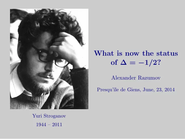
• f ∆ = −1/2?

Alexander Razumov

Presqu’ˆ ıle de Giens, June, 23, 2014

Contents

1 Vertex models 2 Six vertex model 3 XXZ spin chain at ∆ = −1/2 4 General XYZ spin chain

Contents

1 Vertex models 2 Six vertex model 3 XXZ spin chain at ∆ = −1/2 4 General XYZ spin chain

Contents

1 Vertex models 2 Six vertex model 3 XXZ spin chain at ∆ = −1/2 4 General XYZ spin chain

Contents

1 Vertex models 2 Six vertex model 3 XXZ spin chain at ∆ = −1/2 4 General XYZ spin chain

Vertex models

General definitions The playground is a two dimensional square n × m lattice. Each horizontal edge can be in one of ℓ states, and each vertical edge — in

• ne of k states.

The goal is to find the partition function. The partition function is the sum of the Boltzmann weights of all possible states of the lattice. Boltzmann weight of a state is the product of the Boltzmann weights of the vertices.

Vertex models

General definitions The playground is a two dimensional square n × m lattice. Each horizontal edge can be in one of ℓ states, and each vertical edge — in

• ne of k states.

The goal is to find the partition function. The partition function is the sum of the Boltzmann weights of all possible states of the lattice. Boltzmann weight of a state is the product of the Boltzmann weights of the vertices.

Vertex models

General definitions The playground is a two dimensional square n × m lattice. Each horizontal edge can be in one of ℓ states, and each vertical edge — in

• ne of k states.

The goal is to find the partition function. The partition function is the sum of the Boltzmann weights of all possible states of the lattice. Boltzmann weight of a state is the product of the Boltzmann weights of the vertices.

Vertex models

General definitions The playground is a two dimensional square n × m lattice. Each horizontal edge can be in one of ℓ states, and each vertical edge — in

• ne of k states.

The goal is to find the partition function. The partition function is the sum of the Boltzmann weights of all possible states of the lattice. Boltzmann weight of a state is the product of the Boltzmann weights of the vertices.

Vertex models

General definitions The playground is a two dimensional square n × m lattice. Each horizontal edge can be in one of ℓ states, and each vertical edge — in

• ne of k states.

The goal is to find the partition function. The partition function is the sum of the Boltzmann weights of all possible states of the lattice. Boltzmann weight of a state is the product of the Boltzmann weights of the vertices.

Vertex models

Weight of a vertex Boltzmann weigth of a vertex is determined by the states of the adjacent edges. Associate with the states of horizontal edges the indices (a, b, . . .) taking ℓ values, and with the states of vertical edges the indices (i, j, . . .) taking k values. The summation over the states is now the summation over the indices. Monodromy matrix From the weights of the vertices an (ℓ k × ℓ k) matrix in accordance with the picture

Vertex models

Weight of a vertex Boltzmann weigth of a vertex is determined by the states of the adjacent edges. Associate with the states of horizontal edges the indices (a, b, . . .) taking ℓ values, and with the states of vertical edges the indices (i, j, . . .) taking k values. The summation over the states is now the summation over the indices. Monodromy matrix From the weights of the vertices an (ℓ k × ℓ k) matrix in accordance with the picture

a b i j

= Mai|bj

Vertex models

Monodromy matrix for n vertices Sum over the states of internal horizontal edges.

b b b

a c1 c2 cn−1 b i1 i2 i3 in−1 in j1 j2 j3 jn−1 jn

This gives the matrix with the matrix entries Mai1i2...in|bj1j2...jn =

• c1,c2,...,cn−1

Mai1|c1j1Mc1i2|c2j2 . . . Mincn−1|jnb.

Vertex models

Monodromy matrix for n vertices Sum over the states of internal horizontal edges.

b b b

a c1 c2 cn−1 b i1 i2 i3 in−1 in j1 j2 j3 jn−1 jn

This gives the matrix with the matrix entries Mai1i2...in|bj1j2...jn =

• c1,c2,...,cn−1

Mai1|c1j1Mc1i2|c2j2 . . . Mincn−1|jnb.

Vertex models

Transfer matrix Apply the periodic boundary condition in the horizontal direction. Sum over the states of the boundary horizontal edges

b b b

This gives the matrix with the matrix entries Ti1i2...in|j1j2...jn =

• a,c1,c2,...,cn−1

Mai1|c1j1Mc1i2|c2j2 . . . Mincn−1|jna.

Vertex models

Transfer matrix Apply the periodic boundary condition in the horizontal direction. Sum over the states of the boundary horizontal edges

b b b

a c1 c2 cn−1 i1 i2 i3 in−1 in j1 j2 j3 jn−1 jn

This gives the matrix with the matrix entries Ti1i2...in|j1j2...jn =

• a,c1,c2,...,cn−1

Mai1|c1j1Mc1i2|c2j2 . . . Mincn−1|jna.

Vertex models

Transfer matrix Apply the periodic boundary condition in the horizontal direction. Sum over the states of the boundary horizontal edges

b b b

a c1 c2 cn−1 i1 i2 i3 in−1 in j1 j2 j3 jn−1 jn

This gives the matrix with the matrix entries Ti1i2...in|j1j2...jn =

• a,c1,c2,...,cn−1

Mai1|c1j1Mc1i2|c2j2 . . . Mincn−1|jna.

Vertex models

Partition function Applying the periodic boundary condition in the vertical direction we see that Z = tr T m = λm

0 + λm 1 + . . . ,

where λ0 > λ1 > . . . are the eigenvalues of the transfer matrix T. Thermodynamic limit The term thermodynamic limit in the case under consideration means that n, m → ∞. For the free energy for a vertex we have F = 1 mn ln Z = 1 n ln λ0 + 1 mn ln

• 1 +

λ1 λ0 m + . . .

• ≈ 1

n ln λ0.

Vertex models

Partition function Applying the periodic boundary condition in the vertical direction we see that Z = tr T m = λm

0 + λm 1 + . . . ,

where λ0 > λ1 > . . . are the eigenvalues of the transfer matrix T. Thermodynamic limit The term thermodynamic limit in the case under consideration means that n, m → ∞. For the free energy for a vertex we have F = 1 mn ln Z = 1 n ln λ0 + 1 mn ln

• 1 +

λ1 λ0 m + . . .

• ≈ 1

n ln λ0.

Six vertex model

Ice rule For each vertex there are exactly two arrows pointing in and exactly two arrows pointing out. Allowed configurations

Six vertex model

Ice rule For each vertex there are exactly two arrows pointing in and exactly two arrows pointing out. Allowed configurations

Six vertex model

Ice rule For each vertex there are exactly two arrows pointing in and exactly two arrows pointing out. Allowed configurations

Six vertex model

Ice rule For each vertex there are exactly two arrows pointing in and exactly two arrows pointing out. Allowed configurations

Six vertex model

Boltzmann weights Recall that the partition sum is the sum of the Boltzmann weights of all possible configurations of the lattice. The Boltzmann weight of a configuration is the product of the Boltzmann weights of the vertices. Boltzmann weights of the vertices for the six vertex model

Six vertex model

Boltzmann weights Recall that the partition sum is the sum of the Boltzmann weights of all possible configurations of the lattice. The Boltzmann weight of a configuration is the product of the Boltzmann weights of the vertices. Boltzmann weights of the vertices for the six vertex model a a b b c c

Six vertex model

Commuting transfer matrices One can show that [T(a, b, c), T(a′, b′, c′)] = 0 if a2 + b2 − c2 2ab = a′2 + b′2 − c′2 2a′b′ Sectral parameter Standard parametrization a = ρ(qζ − q−1ζ−1), b = ρ(ζ − ζ−1), c = ρ(q − q−1). For this parametrization ∆ = (q + q−1)/2.

Six vertex model

Commuting transfer matrices One can show that [T(a, b, c), T(a′, b′, c′)] = 0 if a2 + b2 − c2 2ab = a′2 + b′2 − c′2 2a′b′ = ∆. Sectral parameter Standard parametrization a = ρ(qζ − q−1ζ−1), b = ρ(ζ − ζ−1), c = ρ(q − q−1). For this parametrization ∆ = (q + q−1)/2.

Six vertex model

Commuting transfer matrices One can show that [T(a, b, c), T(a′, b′, c′)] = 0 if a2 + b2 − c2 2ab = a′2 + b′2 − c′2 2a′b′ = ∆. Sectral parameter Standard parametrization a = ρ(qζ − q−1ζ−1), b = ρ(ζ − ζ−1), c = ρ(q − q−1). For this parametrization ∆ = (q + q−1)/2.

Six vertex model

Commuting transfer matrices One can show that [T(a, b, c), T(a′, b′, c′)] = 0 if a2 + b2 − c2 2ab = a′2 + b′2 − c′2 2a′b′ = ∆. Sectral parameter Standard parametrization a = ρ(qζ − q−1ζ−1), b = ρ(ζ − ζ−1), c = ρ(q − q−1). For this parametrization ∆ = (q + q−1)/2.

Six vertex model

Baxter’s Q-operator Transfer matrices for different values of the spectral parameter commute: [T(ζ), T(ζ′)] = 0. Baxter proved the existence of the (matrix) operator Q(ζ) having the properties [Q(ζ), Q(ζ′)] = 0, [Q(ζ), T(ζ′)] = 0. Baxter TQ-equation The operator equation: T(ζ)Q(ζ) = an(ζ)Q(q−1ζ) + bn(ζ)Q(qζ). The equation for the eigenvalues: λ(ζ)θ(ζ) = an(ζ)θ(q−1ζ) + bn(ζ)θ(qζ).

Six vertex model

Baxter’s Q-operator Transfer matrices for different values of the spectral parameter commute: [T(ζ), T(ζ′)] = 0. Baxter proved the existence of the (matrix) operator Q(ζ) having the properties [Q(ζ), Q(ζ′)] = 0, [Q(ζ), T(ζ′)] = 0. Baxter TQ-equation The operator equation: T(ζ)Q(ζ) = an(ζ)Q(q−1ζ) + bn(ζ)Q(qζ). The equation for the eigenvalues: λ(ζ)θ(ζ) = an(ζ)θ(q−1ζ) + bn(ζ)θ(qζ).

Six vertex model

Baxter’s Q-operator Transfer matrices for different values of the spectral parameter commute: [T(ζ), T(ζ′)] = 0. Baxter proved the existence of the (matrix) operator Q(ζ) having the properties [Q(ζ), Q(ζ′)] = 0, [Q(ζ), T(ζ′)] = 0. Baxter TQ-equation The operator equation: T(ζ)Q(ζ) = an(ζ)Q(q−1ζ) + bn(ζ)Q(qζ). The equation for the eigenvalues: λ(ζ)θ(ζ) = an(ζ)θ(q−1ζ) + bn(ζ)θ(qζ).

Six vertex model

Baxter’s Q-operator Transfer matrices for different values of the spectral parameter commute: [T(ζ), T(ζ′)] = 0. Baxter proved the existence of the (matrix) operator Q(ζ) having the properties [Q(ζ), Q(ζ′)] = 0, [Q(ζ), T(ζ′)] = 0. Baxter TQ-equation The operator equation: T(ζ)Q(ζ) = an(ζ)Q(q−1ζ) + bn(ζ)Q(qζ). The equation for the eigenvalues: λ(ζ)θ(ζ) = an(ζ)θ(q−1ζ) + bn(ζ)θ(qζ).

Six vertex model

The special value of the parameter q For q = exp(±2πi/3) (∆ = −1/2) there are some reasonings for the existence of a solution to the TQ-equation with λ(ζ) = −(q−1ζ − qζ−1)n. In this case for the function ϕ(ζ) = (q−1ζ − qζ−1)nθ(ζ) TQ-equation takes the form ϕ(ζ) + ϕ(qζ) + ϕ(q2ζ) = 0. An explicit solution to this equation was found by Yuri Stroganov

• Yu. G. Stroganov, The importance of being odd, J. Phys. A: Math. Gen. 34

(2001) L179-L185.

Six vertex model

The special value of the parameter q For q = exp(±2πi/3) (∆ = −1/2) there are some reasonings for the existence of a solution to the TQ-equation with λ(ζ) = −(q−1ζ − qζ−1)n. In this case for the function ϕ(ζ) = (q−1ζ − qζ−1)nθ(ζ) TQ-equation takes the form ϕ(ζ) + ϕ(qζ) + ϕ(q2ζ) = 0. An explicit solution to this equation was found by Yuri Stroganov

• Yu. G. Stroganov, The importance of being odd, J. Phys. A: Math. Gen. 34

(2001) L179-L185.

Six vertex model

The special value of the parameter q For q = exp(±2πi/3) (∆ = −1/2) there are some reasonings for the existence of a solution to the TQ-equation with λ(ζ) = −(q−1ζ − qζ−1)n. In this case for the function ϕ(ζ) = (q−1ζ − qζ−1)nθ(ζ) TQ-equation takes the form ϕ(ζ) + ϕ(qζ) + ϕ(q2ζ) = 0. An explicit solution to this equation was found by Yuri Stroganov

• Yu. G. Stroganov, The importance of being odd, J. Phys. A: Math. Gen. 34

(2001) L179-L185.

XXZ spin chain at ∆ = −1/2

Connection to the six vertex model The Hamiltonian of the XXZ spin chain HXXZ = −1 2

n

• k=1

[σx

kσx k+1 + σy kσy k+1 + ∆σz kσz k+1]

is connected to the transfer matrix of the six vertex model as follows: T(ζ)dT(ζ) dζ

• ζ=1

= − 2 q − q−1

• HXXZ − n∆

2

• .

It follows from this equality that [HXXZ, T(ζ)] = 0 At ∆ = −1/2, if an eigenvector of the transfer matrix with the eigenvalue λ(ζ) = −(q−1ζ − qζ−1)n exists it is an eigenvector of the Hamiltonian HXXZ with the eigenvalue E = −3n/4.

XXZ spin chain at ∆ = −1/2

Mathematica enters the game It was demonstrated that an eigenvector of the Hamiltonian HXXZ with the eigenvalue E = −3n/4 exists for ∆ = −1/2 for odd n = 1, 3, . . . , 17. For even n = 2, 4, . . . , 16 there is no such vector. These results are given in the paper

• A. V. Razumov and Yu. G. Stroganov, Spin chains and combinatorics, J. Phys.

A: Math. Gen. 34 (2001) 31853190. In the same paper a few conjectures on the properties of the eigenvector are formulated.

XXZ spin chain at ∆ = −1/2

Mathematica enters the game It was demonstrated that an eigenvector of the Hamiltonian HXXZ with the eigenvalue E = −3n/4 exists for ∆ = −1/2 for odd n = 1, 3, . . . , 17. For even n = 2, 4, . . . , 16 there is no such vector. These results are given in the paper

• A. V. Razumov and Yu. G. Stroganov, Spin chains and combinatorics, J. Phys.

A: Math. Gen. 34 (2001) 31853190. In the same paper a few conjectures on the properties of the eigenvector are formulated.

XXZ spin chain at ∆ = −1/2

Conjecture 1 The ground state of the Hamiltonian HXXZ|∆=−1/2 for odd n has the energy −3n/4. Proof

• X. Yang and P. Fendley, Non-local space-time supersymmetry on the lattice, J.
• Phys. A: Math. Gen. 37 (2004) 8937-48;
• G. Veneziano and J. Wosiek, A supersymmetric matrix model: III. Hidden

SUSY in statistical systems, JHEP 11 (2006) 030.

XXZ spin chain at ∆ = −1/2

Conjecture 2 If one divides the components of the ground state vector by the component with minimal absolute value all other components become positive integers. Here the maximal component for n = 2m + 1 coincides with the number Am of the alternating sign matrices of order m. Proof

• A. V. Razumov, Yu. G. Stroganov and P. Zinn–Justin, Polynomial solutions of

qKZ equation and ground state of XXZ spin chain at ∆ = −1/2, J. Phys. A:

• Math. Theor. 40 (2007) 11827-11847.

XXZ spin chain at ∆ = −1/2

Definition An m × m matrix satisfying the conditions all matrix entries are either 0 or +1 or −1 +1 and −1 alternates in every row and every column the first and the last nonzero entry in every row and every column is +1 is called an alternating sign matrix of order m. All alternating-sign matrices of order 3   +1 0 +1 0 +1     +1 0 +1 0 +1     0 +1 0 +1 +1     0 +1 +1 0 +1     0 +1 +1 0 +1     0 +1 0 +1 +1     0 +1 +1 −1 +1 0 +1  

XXZ spin chain at ∆ = −1/2

Conjecture 3 With the above normalization, the sum of squared components of the ground state vector is N 2

m and the the sum of the components is 3m/2Nm, where

Nm = 3m/2 2m 2 · 5 · · · (3m − 1) 1 · 3 · · · (2m − 1)Am. Proof

• P. Di Francesco, P. Zinn–Justin and J.–B. Zuber, Sum rules for the ground

states of the O(1) loop model on a cylinder and the XXZ spin chain, J. Stat. Phys.: Theor. Exp. (2006) P08011.

XXZ spin chain at ∆ = −1/2

To study the correlation functions it is convenient to use the operators αk = (1 + σz

k)/2.

Conjecture 4 The emptiness formation probabilities satisfy the equality α1 · · · αp−1 α1 · · · αp−1αp = (2p − 2)!(2p − 1)!(2m + p)!(m − p)! (p − 1)!(3p − 2)!(2m − p + 1)!(m + p − 1)!. Proof

• N. Kitanine, J. M. Maillet, N. A. Slavnov and V. Terras, Emptiness formation

probability of the XXZ spin-1 / 2 Heisenberg chain at ∆ = 1/2, J. Phys. A:

• Math. Gen. 35 (2002) L385-L388.
• L. Cantini, Finite size emptiness formation probability of the XXZ spin chain at

∆ = −1/2, J. Phys. A: Math. Theor. 45 (2012) 135207.

General XYZ spin chain

Hamiltonian of XYZ spin chain HXYZ = −1 2

n

• j=1

[Jxσx

kσx k+1 + Jyσy kσy k+1 + Jzσz kσz k+1]

The periodic boundary conditions σx

n+1 = σx 1,

σy

n+1 = σy 1,

σz

n+1 = σz 1.

Baxter’s observation Baxter observed that the case JxJy + JxJz + JyJz = 0 is very special. For XXZ spin chain Jx = 1, Jy = 1, Jz = ∆, and the above equality takes the form ∆ = −1/2.

General XYZ spin chain

Hamiltonian of XYZ spin chain HXYZ = −1 2

n

• j=1

[Jxσx

kσx k+1 + Jyσy kσy k+1 + Jzσz kσz k+1]

The periodic boundary conditions σx

n+1 = σx 1,

σy

n+1 = σy 1,

σz

n+1 = σz 1.

Baxter’s observation Baxter observed that the case JxJy + JxJz + JyJz = 0 is very special. For XXZ spin chain Jx = 1, Jy = 1, Jz = ∆, and the above equality takes the form ∆ = −1/2.

General XYZ spin chain

References for the case of XYZ spin chain I

• Yu. G. Stroganov, The 8-vertex model with a special value of the crossing

parameter and the related XYZ spin chain, Integrable Structures of Exactly Solvable Two-Dimensional Models of Quantum Field Theory (S. Pakulyak and

• G. von Gehlen, eds.), Kluwer, Dortrecht, 2001, pp. 315–319
• V. V. Bazhanov and V. V. Mangazeev, Eight-vertex model and non-stationary

Lam´ e equation, J. Phys. A: Math. Gen. 38 (2005), L145–L153

• V. V. Bazhanov and V. V. Mangazeev, The eight-vertex model and Painlev´

e VI,

• J. Phys. A: Math. Gen. 39 (2006), 12235–12243
• V. V. Bazhanov and V. V. Mangazeev, The eight-vertex model and Painlev´

e VI equation II: eigenvector results, J. Phys. A: Math. Gen. 43 (2010), 085206 (16pp)

• A. V. Razumov and Yu. G. Stroganov, A possible combinatorial point for the

XYZ spin chain, Theor. Math. Phys. 164 (2010) 977–991

• P. Zinn-Justin, Sum rule for the eight-vertex model on its combinatorial line,

Symmetries, Integrable Systems and Representations, Springer, 2013, pp. 599–637

General XYZ spin chain

References for the case of XYZ spin chain II

• C. Hagendorf and P. Fendley, Exact and simple results for the XYZ and strongly

interacting fermion chains, J. Phys. A: Math. Theor. 43 (2010) 402004 (8pp)

• C. Hagendorf and P. Fendley, Ground-state properties of a supersymmetric

fermion chain, J. Stat. Mech. (2011) P02014 (22pp)

• C. Hagendorf and P. Fendley, The eight-vertex model and lattice

supersymmetry, J. Stat. Phys. 146 (2012) 1122-1155

• C. Hagendorf, Spin chains with dynamical lattice supersymmetry, J. Stat. Phys.

150 (2013) 609–657

• H. Rosengren, Special polynomials related to the supersymmetric eight-vertex
• model. I. Behaviour at cusps, arXiv:1305.0666
• H. Rosengren, Special polynomials related to the supersymmetric eight-vertex
• model. II. Schr¨
• dinger equation, arXiv:1312.5879
• H. Rosengren, Special polynomials related to the supersymmetric eight-vertex
• model. III. Painlev´

e VI equation, arXiv:1405.5318