What is an experiment? In an experiment, a Physical Phenomenon is - PowerPoint PPT Presentation

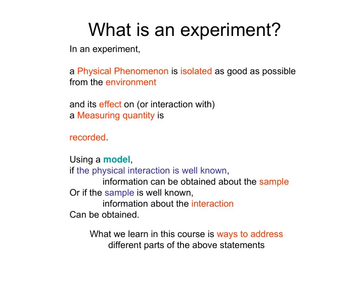
What is an experiment? In an experiment, a Physical Phenomenon is isolated as good as possible from the environment and its effect on (or interaction with) a Measuring quantity is recorded. Using a model , if the physical interaction is well known, information can be obtained about the sample Or if the sample is well known, information about the interaction Can be obtained. What we learn in this course is ways to address different parts of the above statements

What is an experiment? In an experiment, The effect induces changes on the Measured quantity. Because absolute measurements are either hard or impossible, we look at differences (or changes) in the measured quantity most of the time. Example: • plot temperature as a function of Time. • measure current as a function of voltage • measure luminescence as a function of wavelength

Signals and Noise • In the broadest sense, a signal is – A time varying quantity, or, – A sequence of numbers • In information theory – A signal is a sequence of numbers carrying a message (coded with an alphabet) • Noise is an unintended (unwanted) and random addition to the signal that can not be separated from the signal

Signal and Noise example noise interference

Example : Sinusoidal and Noise Original sinusoid Example Original sinusoid + added noise Oscilloscope traces time

Why can’t we separate the noise? • Noise is RANDOM, i.e. we don’t know it a priori . And we can not estimate it perfectly. (otherwise it wouldn’t be noise, but some sort of interference) “ I will give you 50 + (a random number between -50 and 50) YTL” “I can not decide if I will be happy or not! The amount can be 0 to 100 YTL. ”

How strong the noise is compared to the signal makes a difference. “ I will give you 50 + (a random number between -5 and 5) YTL” “The amount can be 45 to 55 YTL. I have a better idea of how much you will give me!”

Signal to Noise Ratio Informal, verbal definition: Signal – to – Noise Ratio (SNR) Signal Power SNR = Noise Power Generally we want as high an SNR as possible. This makes our measurement result more accurate

Signal to Noise Ratio Signal Power ~ 1 In this case SNR = Noise Power noise signal The limit of our measurement is the noise level. A measurement with SNR ~ 1 is barely acceptable

We measure Voltages (most of the time anyways) • For pedagogical reasons, during the discussion of noise and signals, we will use voltages and currents. • Other signals and noise sources can be understood easily by extending your understanding of voltage and current waveforms.

Noise and Random Numbers Signal + Noise = Measurement Result We want to This is a random We know this one know this one number We have to refresh our memory about random numbers

Discrete Random Numbers (variables) • A series of numbers X – Gives a different outcome for each trial – Trials are INDEPENDENT of each other Trial number 1 X 1 =1 2 X 2 =3 3 X 3 =2 4 X 4 =5 ……….

Discrete Random Variables • A series of numbers X n – Results of trials take values from a set (the space of outcomes, Ω ) X n is an element of Ω ={ 1,2,3,4,5,6 } Each outcome value has a probability assigned to it, p i

Uniformly Distributed Random Var. X n is an element of Example Ω ={ 1,2,3,4,5,6 } ∑ = P 1 = 1/6 1 p i P 2 = 1/6 i P 3 = 1/6 Probabilities add up to 1 P 4 = 1/6 P 5 = 1/6 P 6 = 1/6

Uniformly Distributed Random Var. X n is an element of Example Ω ={ 0,1 } 0 1 P 0 = ½ P 1 = ½

Concept of Probability Distribution X n is an element of Ω ={ 1,2,3,4,5,6 } ∑ = 1 p i i Probability mass function P 1 = 1/6, P 2 = 1/6, P 3 = 1/6, P 4 = 1/6, P 5 = 1/6, P 6 = 1/6

Expected value of a Random Variable Different Notations can be used E(X) = μ <X> = μ “Expected value of X is μ ”

Expected value of a Random Variable ∑ E(X) = μ μ = p i X i <X> = μ Weighted average of outcomes, using probabilites as weights Expectation shows the “center of mass” of the probability distribution For the dice outcomes, μ = 3.5

Variance of a Random Variable σ x2 =E((X- μ ) 2 ) σ x2 = <X 2> -<X> 2 Variance is a measure of the width of the Probability distribution

Variance of a Random Variable σ x2 = <X 2 >-<X> 2 σ x is very closely related to the noise amplitude

Standart Deviation σ x2 = <X 2> -<X> 2

Binomial Distribution 1 0 P 0 = p P 1 = q =1-p Binomial coin toss with an unbalanced coin. You toss it N times. And count the number of heads. Your result X is the number of heads.

Binomial Distribution Number Number Prob. 1 0 of 1s of 1s 0 1/16 1/16 = q*q*q*q 0 0 0 0 0 1 4/16 P 0 = p P 1 = q =1-p 1/16 = q*q*q*p 0 0 0 1 1 2 6/16 1/16 = q*q*p*q 0 0 1 0 1 p=q=1/2 3 4/16 1/16 0 0 1 1 2 4 1/16 1/16 0 1 0 0 1 Example : 4 trials. 1/16 0 1 0 1 2 Increasing number of trials 1/16 0 1 1 0 2 1/16 0 1 1 1 3 1/16 1 0 0 0 1 1/16 1 0 0 1 2 1/16 1 0 1 0 2 1/16 1 0 1 1 3 1/16 1 1 0 0 2 1/16 1 1 0 1 3 1/16 1 1 1 0 3 1/16 1 1 1 1 4

Binomial Distribution p=0.5 q=0.5 p=0.01 q=0.99 Increasing number of trials In the limit of large number of trials: Changes between a Gaussian 1 0 And something like an exponential Depending on p and q ! P 0 = p P 1 = q =1-p

Discrete and Continous Distributions Outcomes are discrete numbers Outcomes are Real numbers Probability Mass function Probability Distribution function ∑ μ = p i X i

Continous Distributions Probability that the outcome is between x and x+dx dP = f(x)dx Probability Distribution function Outcomes are Real numbers

Normal Distribution and Binomial Distribution There is a special relation between Binomial and Gaussian distributions. Gaussian is a limit for the binomial is p is about 0.5, and number of trials is large.

Poisson Distribution and Binomial Distribution There is a special relation between Binomial and Poisson distributions. Poisson is a limit for the binomial is N*p is small, and number of trials is large (p<<1). Probability Mass function Important because electrons and photons are quantized (discrete). If we measure them at regular intervals, we are counting the success events.

Normal Distribution and Central Limit Theorem So important that Gauss appears on the German Mark

Normal Distribution and the Central Limit Theorem The sum of a large number of arbitrary random variables converge to a gaussian distribution. • The convergence can be rather quick. • This theorem explains why X Gaussian Distributed Noise Y= X1+X2 is commonly observed. We skip the proof, can be found elsewhere (wikipedia etc.) K=X1+X2+X3+X4 Z=X1+X2+X3

Mean and Variance of Random Variables upon addition Gaussian ( Normal ) Random Variable

Observations 1. Addition of a Constant signal to the Random Variable Does not increase the variance. 2. Multiplication by a constant number multiplies the variance as well

Observations 1. Addition of two Random Variables adds the means linearly. 2. Standard Deviations are added in the second order. 3. Addition of N Random variables of same distribution with mean μ and standard deviation σ results in μ s = N μ σ s = σ√ N

Observations 1. Subtraction increases the Standard Deviation just like addition does, Subtracting two noisy waveforms does not clear the noise.

Averaging

Ensemble Averaging Ensemble of experiments: N Copies of the same system Each having its own noise (but same distribution)

Averaging μ s = N μ σ s = σ√ N If SNR is defined as μ / σ Then by making multiple measurements and adding the results we get μ s / σ s = N μ / σ√ N = ( μ / σ ) √ N There is an improvement in the SNR!