WHAT CANNOT BE SOLVED BY THE ELLIPSOID METHOD? Albert Atserias - PowerPoint PPT Presentation
WHAT CANNOT BE SOLVED BY THE ELLIPSOID METHOD? Albert Atserias Universitat Polit` ecnica de Catalunya Barcelona convex programming finite model theory and descriptive complexity approximation algorithms and computational complexity Part I
WHAT CANNOT BE SOLVED BY THE ELLIPSOID METHOD? Albert Atserias Universitat Polit` ecnica de Catalunya Barcelona
convex programming finite model theory and descriptive complexity approximation algorithms and computational complexity
Part I ELLIPSOID METHOD
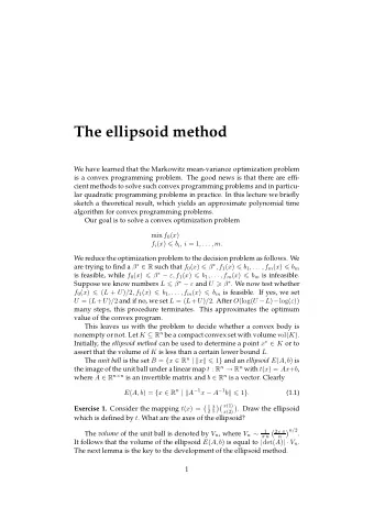
The Ellipsoid Method • Invented for non-linear convex optimization over R n in 1970’s. • Adapted to linear programming (LP) by Khachiyan in 1979. A x = b , x ≥ 0 Feasibility: c T x Optimization: max s.t. A x = b , x ≥ 0 . • First poly-time algorithm for LP: solved a big theoretical problem. • Time poly in size( A ) , size( b ) , size( c ) in bit-model of computation.
Problem Statement Given : a convex P ⊆ R n and an accuracy parameter ǫ > 0 . Goal : find some point x in P . Assumptions : • promise that P ⊆ S ( 0 , R ) for some known R > 0 , • promise that S ( x 0 , r ) ⊆ P for some unknown x 0 and r > 0 , • promise that a separation oracle for P is available.
Algorithm and Convergence Start : P ⊆ E 0 := S (0 , R ) Steps : i = 0 , 1 , 2 , . . . � � 1 Progress : vol( E i +1 ) ≤ 1 − vol( E i ) poly( n ) Terminate : either center( E i ) ∈ P or vol( E i ) ≤ vol( S ( x 0 , r ))
Geometric Basis for Progress Measure The L¨ owner-John ellipsoid Theorem : For every convex P ⊆ R n , there is a unique ellipsoid E of minimial volume containing K . Moreover, K contains E shrinked by a factor of n .
Linear and Semidefinite Programming (LP and SDP) maximize � c , x � � a j , x � = b j , j ∈ [ m ] subject to x ≥ 0
Linear and Semidefinite Programming (LP and SDP) maximize � c , x � � a j , x � = b j , j ∈ [ m ] subject to x ≥ 0 maximize � C , X � � A j , X � = b j , j ∈ [ m ] subject to X is positive semi-definite (PSD)
Linear and Semidefinite Programming (LP and SDP) maximize � c , x � � a j , x � = b j , j ∈ [ m ] subject to x ≥ 0 maximize � C , X � � A j , X � = b j , j ∈ [ m ] subject to � A , X � ≥ 0 , A ∈ PSD
Part II LP AND SDP FOR COMBINATORICS
Vertex cover Problem: Given an undirected graph G = ( V, E ) , find the smallest number of vertices that touches every edge. Notation: vc( G ) . Observe: A ⊆ V is a vertex cover of G iff V \ A is an independent set of G
Linear programming relaxation LP relaxation: minimize � u ∈ V x u subject to x u + x v ≥ 1 for every ( u, v ) ∈ E, x u ≥ 0 for every u ∈ V. Notation: fvc( G ) .
Approximation Approximation: fvc( G ) ≤ vc( G ) ≤ 2 · fvc( G ) Integrality gap: vc( G ) sup fvc( G ) G
Approximation Approximation: fvc( G ) ≤ vc( G ) ≤ 2 · fvc( G ) Integrality gap: vc( G ) sup fvc( G ) = 2 . G
Approximation Approximation: fvc( G ) ≤ vc( G ) ≤ 2 · fvc( G ) Integrality gap: vc( G ) sup fvc( G ) = 2 . G Gap examples: 1. vc( K n ) = n − 1 , 2. fvc( K n ) = 1 2 n .
LP tightenings Add triangle inequalities: minimize � u ∈ V x u subject to x u + x v ≥ 1 for every ( u, v ) ∈ E, x u ≥ 0 for every u ∈ V, x u + x v + x w ≥ 2 for every triangle { u, v, w } in G.
LP tightenings Add triangle inequalities: minimize � u ∈ V x u subject to x u + x v ≥ 1 for every ( u, v ) ∈ E, x u ≥ 0 for every u ∈ V, x u + x v + x w ≥ 2 for every triangle { u, v, w } in G. Integrality gap: Remains 2 . Gap examples: Triangle-free graphs with small independence number.
LP and SDP Hierarchies Hierarchy: Systematic ways of generating all linear inequalities that are valid over the integral hull.
LP and SDP Hierarchies Hierarchy: Systematic ways of generating all linear inequalities that are valid over the integral hull. Given a polytope: P = { x ∈ R n : Ax ≥ b } , P Z = convexhull { x ∈ { 0 , 1 } n : Ax ≥ b } .
LP and SDP Hierarchies Hierarchy: Systematic ways of generating all linear inequalities that are valid over the integral hull. Given a polytope: P = { x ∈ R n : Ax ≥ b } , P Z = convexhull { x ∈ { 0 , 1 } n : Ax ≥ b } . Produce explicit nested polytopes: P = P 1 ⊇ P 2 ⊇ · · · ⊇ P n − 1 ⊇ P n = P Z
P k : SDP Hierarchy (Lasserre/SOS Hierarchy)
P k : SDP Hierarchy (Lasserre/SOS Hierarchy) Given linear inequalities L 1 ≥ 0 , . . . , L m ≥ 0
P k : SDP Hierarchy (Lasserre/SOS Hierarchy) Given linear inequalities L 1 ≥ 0 , . . . , L m ≥ 0 produce all linear inequalities of the form m n � � ( x 2 Q 0 + L j Q j + i − x i ) Q i = L ≥ 0 j =1 i =1
P k : SDP Hierarchy (Lasserre/SOS Hierarchy) Given linear inequalities L 1 ≥ 0 , . . . , L m ≥ 0 produce all linear inequalities of the form m n � � ( x 2 Q 0 + L j Q j + i − x i ) Q i = L ≥ 0 j =1 i =1 where � Q 2 Q j = with jℓ ℓ ∈ I
P k : SDP Hierarchy (Lasserre/SOS Hierarchy) Given linear inequalities L 1 ≥ 0 , . . . , L m ≥ 0 produce all linear inequalities of the form m n � � ( x 2 Q 0 + L j Q j + i − x i ) Q i = L ≥ 0 j =1 i =1 where � Q 2 Q j = with jℓ ℓ ∈ I and deg( Q 0 ) , deg( L j Q j ) , deg(( x 2 i − x i ) Q i ) ≤ k .
P k : SDP Hierarchy (Lasserre/SOS Hierarchy) Given linear inequalities L 1 ≥ 0 , . . . , L m ≥ 0 produce all linear inequalities of the form m n � � ( x 2 Q 0 + L j Q j + i − x i ) Q i = L ≥ 0 j =1 i =1 where � Q 2 Q j = with jℓ ℓ ∈ I and deg( Q 0 ) , deg( L j Q j ) , deg(( x 2 i − x i ) Q i ) ≤ k . Then: P k = { x ∈ R n : L ( x ) ≥ 0 for each produced L ≥ 0 }
P k : LP Hierarchy (Sherali-Adams Hierarchy) Given linear inequalities L 1 ≥ 0 , . . . , L m ≥ 0 produce all linear inequalities of the form m n � � ( x 2 Q 0 + L j Q j + i − x i ) Q i = L ≥ 0 j =1 i =1 where � � � Q i = c ℓ x i (1 − x i ) with c ℓ ≥ 0 ℓ ∈ J i ∈ A ℓ i ∈ B ℓ and deg( Q 0 ) , deg( L j Q j ) , deg(( x 2 i − x i ) Q i ) ≤ k . Then: P k = { x ∈ R n : L ( x ) ≥ 0 for each produced L ≥ 0 }
Example: triangles in P 3 For each triangle { u, v, w } in G : Q 0 + ( x u + x v − 1) Q 1 + ( x u + x w − 1) Q 2 + ( x v + x w − 1) Q 3 + ( x 2 u − x u ) Q 4 + ( x 2 v − x v ) Q 5 + ( x 2 w − x w ) Q 6 = ? ( x u + x v + x w − 2) . Q i = a i + b i x u + c i x v + d i x w + e i x u x v + f i x u x w + g i x v x w + h i x u x v x w
Solving P k Lift-and-project : • Step 1: lift from R n up to R ( n +1) k and linearize the problem • Step 2: project from R ( n +1) k down to R n Proposition : Optimization of linear functions over P k can be solved in time † m O (1) n O ( k ) . Proof : 1. for LP- P k : by linear programming 2. for SDP- P k : by semidefinite programming
An Important Open Problem Define sa k fvc( G ) : optimum fractional vertex cover of LP- P k sdp k fvc( G ) : optimum fractional vertex cover of SDP- P k Open problem: vc( G ) ? sup < 2 sdp 4 fvc( G ) G
What’s Known
What’s Known Known (conditional hardness): • 1 . 0001 -approximating vc( G ) is NP-hard by PCP Theorem • 1 . 36 -approximating vc( G ) is NP-hard • 2 -approximating vc( G ) is NP-hard assuming UGC
What’s Known Known (conditional hardness): • 1 . 0001 -approximating vc( G ) is NP-hard by PCP Theorem • 1 . 36 -approximating vc( G ) is NP-hard • 2 -approximating vc( G ) is NP-hard assuming UGC Known (unconditional hardness): • sup G vc( G ) / sa k fvc( G ) = 2 for any k = n o (1) • sup G vc( G ) / sdp - fvc( G ) = 2 • variants: pentagonal, antipodal triangle, local hypermetric, ...
What’s Known Known (conditional hardness): • 1 . 0001 -approximating vc( G ) is NP-hard by PCP Theorem • 1 . 36 -approximating vc( G ) is NP-hard • 2 -approximating vc( G ) is NP-hard assuming UGC Known (unconditional hardness): • sup G vc( G ) / sa k fvc( G ) = 2 for any k = n o (1) • sup G vc( G ) / sdp - fvc( G ) = 2 • variants: pentagonal, antipodal triangle, local hypermetric, ... Gap examples: odl Graphs: FR n γ = ( F n 2 , {{ x, y } : x + y ∈ A n Frankl-R¨ γ } ) .
What’s Known Known (conditional hardness): • 1 . 0001 -approximating vc( G ) is NP-hard by PCP Theorem • 1 . 36 -approximating vc( G ) is NP-hard • 2 -approximating vc( G ) is NP-hard assuming UGC Known (unconditional hardness): • sup G vc( G ) / sa k fvc( G ) = 2 for any k = n o (1) • sup G vc( G ) / sdp - fvc( G ) = 2 • variants: pentagonal, antipodal triangle, local hypermetric, ... Gap examples: odl Graphs: FR n γ = ( F n 2 , {{ x, y } : x + y ∈ A n Frankl-R¨ γ } ) . [Dinur, Safra, Khot, Regev, Kleinberg, Charikar, Hatami, Magen, Georgiou, Lovasz, Arora, Alekhnovich, Pitassi; 2000’s]
Part III COUNTING LOGIC
Bounded-Variable Logics First-order logic of graphs : E ( x, y ) : x and y are joined by an edge x = y : x and y denote the same vertex ¬ φ : negation of φ holds φ ∧ ψ : both φ and ψ hold ∃ x ( φ ) : there exists a vertex x that satisfies φ
Bounded-Variable Logics First-order logic of graphs : E ( x, y ) : x and y are joined by an edge x = y : x and y denote the same vertex ¬ φ : negation of φ holds φ ∧ ψ : both φ and ψ hold ∃ x ( φ ) : there exists a vertex x that satisfies φ First-order logic with k variables (or width k ) : L k : collection of formulas for which all subformulas have at most k free variables.
Recommend
More recommend
Explore More Topics
Stay informed with curated content and fresh updates.


