Week 8: Classification & Model Building Classification for - PowerPoint PPT Presentation
BUS41100 Applied Regression Analysis Week 8: Classification & Model Building Classification for Binary Outcomes, Variable Selection, BIC, AIC, LASSO Max H. Farrell The University of Chicago Booth School of Business Classification A common
BUS41100 Applied Regression Analysis Week 8: Classification & Model Building Classification for Binary Outcomes, Variable Selection, BIC, AIC, LASSO Max H. Farrell The University of Chicago Booth School of Business
Classification A common goal with logistic regression is to classify the inputs depending on their predicted response probabilities. Example: evaluating the credit quality of (potential) debtors. ◮ Take a list of borrower characteristics. ◮ Build a prediction rule for their credit. ◮ Use this rule to automatically evaluate applicants (and track your risk profile). You can do all this with logistic regression, and then use the predicted probabilities to build a classification rule. ◮ A simple classification rule would be that anyone with ˆ P (good | x ) > 0 . 5 can get a loan, and the rest cannot. —————— 1 (Classification is a huge field, we’re only scratching the surface here.)
We have data on 1000 loan applicants at German community banks, and judgment of the loan outcomes (good or bad). The data has 20 borrower characteristics, including ◮ credit history (5 categories), ◮ housing (rent, own, or free), ◮ the loan purpose and duration, ◮ and installment rate as a percent of income. Unfortunately, many of the columns in the data file are coded categorically in a very opaque way. (Most are factors in R.) 2
Logistic regression yields ˆ P [good | x ] = ˆ P [ Y = 1 | x ] : > full <- glm(GoodCredit~., family=binomial, data=credit) > predfull <- predict(full, type="response") Need to compare to binary Y = { 0 , 1 } . ◮ Convert: ˆ Y = 1 { ˆ P [ Y = 1 | x ] > 0 . 5 } ◮ classification error: Y i − ˆ Y i = {− 1 , 0 , 1 } . > errorfull <- credit[,1] - (predfull >= .5) > table(errorfull) -1 0 1 74 786 140 > mean(abs(errorfull)) ## add weights if you want [1] 0.214 > mean(errorfull^2) [1] 0.214 3
ROC & PR curves Is one type of mistake worse than the other? ◮ You’ll want to have ˆ P > 0 . 5 of a “positive” outcome before taking a risky action. ◮ You decide which error is worse, and by how much. > table(credit[,1] - (predfull >= .6) -1 0 1 40 789 171 > mean((credit[,1] - (predfull >= .6))^2) [1] 0.211 What happens as the cut-off varies? What’s the “best” cut-off? To answer we can use two curves: 1. ROC: Receiver Operating Characteristic 2. PR: Precision-Recall 4
> library("pROC") > roc.full <- roc(credit[,1] ~ predfull) > coords(roc.full, x=0.5) threshold specificity sensitivity 0.5000000 0.8942857 0.5333333 > coords(roc.full, "best") threshold specificity sensitivity 0.3102978 0.7614286 0.7700000 1.0 Sensitivity 0.8 Y true positive rate Sensitivity 0.6 X Specificity 0.4 true negative rate 0.2 —————— X cut−off = 0.5 Many related names: hit rate, fall-out Y cut−off = best 0.0 false discovery rate, . . . 1.0 0.8 0.6 0.4 0.2 0.0 Specificity 5
> library("PRROC") > pr.full <- pr.curve(scores.class0=predfull, + weights.class0=credit[,1], curve=TRUE) 1.0 Recall 0.8 true positive rate 0.8 0.6 same as senstivity Precision 0.6 0.4 Precision 0.4 positive predictive value 0.2 0.2 —————— 0.0 0.0 Many related names: hit rate, fall-out 0.0 0.2 0.4 0.6 0.8 1.0 false discovery rate, . . . Recall 6
Now we know how to evaluate a classification model, so we can compare models. But which models should we compare? > empty <- glm(GoodCredit~1, family=binomial, data=credit) > history <- glm(GoodCredit~history3, family=binomial, data=credit) Misclassification rates: > c(empty=mean(abs(errorempty)), + history=mean(abs(errorhistory)), + full=mean(abs(errorfull)) ) empty history full 0.300 0.283 0.214 Why is this both obvious and not helpful? 7
A word of caution Why not just throw everything in there? > too.good <- glm(GoodCredit~. + .^2, family=binomial, + data=credit) Warning messages: 1: glm.fit: algorithm did not converge 2: glm.fit: fitted probabilities numerically 0 or 1 occurred This warning means you have the logistic version of our “connect the dots” model. ◮ Just as useless as before! > c(empty=mean(abs(errorempty)), + history=mean(abs(errorhistory)), + full=mean(abs(errorfull)) , + too.good=mean(abs(errortoo.good)) ) empty history full too.good 0.300 0.283 0.214 0.000 8
Model Selection Our job now is to pick which X variables belong in our model. ◮ A good prediction model summarizes the data but does not overfit. What if the goal isn’t just prediction? ◮ A good model answers the question at issue. ◮ Better predictions don’t matter if the model doesn’t answer the question. ◮ A good regression model obeys our assumptions. ◮ Especially important when the goal is inference/relationships. ◮ A causal model is only good when it meets even more assumptions. 9
What is the goal? 1. Relationship-type questions and inference? ◮ Are women paid differently than men on average? > lm(log.WR ~ sex) ◮ Does age/experience differently affect men and women? > lm(log.WR ~ age*sex - sex) ◮ No other models matter 2. Data summarization? ◮ In time series we matched the dynamics/trends, and stopped there. 3. Prediction? ◮ Need a fair, objective criterion that matches the idea of predicting the future. Avoid overfitting. 10
Overfitting We have already seen overfitting twice: 1. Week 5: R 2 ↑ as more variables went into MLR > c(summary(trucklm1)$r.square, summary(trucklm3)$r.square, + summary(trucklm6)$r.square) [1] 0.021 0.511 0.693 2. Just a minute ago: Classification error ↓ as more variables into logit empty history full 0.300 0.283 0.214 Fitting the data at hand better and better . . . but getting worse at predicting the next observation. How can we use the data to pick the model without relying on the data too much? 11
Out-of-sample prediction How do we evaluate a forecasting model? ◮ Make predictions! ◮ Out-of-sample prediction error is the Gold Standard for comparing models. (If what you care about is prediction.) Basic Idea: We want to use the model to forecast outcomes for observations we have not seen before. ◮ Use the data to create a prediction problem. ◮ See how our candidate models perform. We’ll use most of the data for training the model, and the left over part for validating/testing it. 12
In a validation scheme, you ◮ fit a bunch of models to most of the data (training set) ◮ choose the one performing best on the rest (testing set). For each model: ◮ Obtain b 0 , . . . , b d on the training data. ◮ Use the model to obtain fitted values for the n test testing data points: ˆ j b or ˆ Y j = 1 { ˆ Y j = x ′ P [ Y =1 | x j ] > 0 . 5 } ◮ Calculate the Mean Square Error for these predictions. n test 1 � ( Y j − ˆ Y j ) 2 MSE = n test j =1 13
Out of sample validation steps: 1) Split the data into testing/training samples. > set.seed(2) > train.samples <- sample.int(nrow(credit), 0.95*nrow(credit)) > train <- credit[train.samples,] > test <- credit[-train.samples,] 2) Fit models on the training data > full <- glm(GoodCredit~., family=binomial, data=train) > history <- glm(GoodCredit~history3, family=binomial, data=train 3) Predict on the test data > predfull <- predict(full, type="response", newdata=test) > errorfull <- test[,"GoodCredit"] - (predfull >= .5) 4) Compute MSE/MAE > c(empty=mean(errorempty^2), history=mean(errorhistory^2), + full=mean(errorfull^2) , too.good=mean(errortoo.good^2) ) empty history full too.good 14 0.24 0.20 0.32 0.42
This missing piece is in 2) Fit models on the training data Which models? The rest of these slides are about tools to help with choosing models. We’ll do linear and logistic examples. ◮ Once we have tools for step 2, it’s easy to compute out-of-sample MSE. There are two pieces to the puzzle: ◮ Select the “universe of variables” ◮ Choose the best model(s) The computer helps only with the 2 nd ! 15
The universe of variables is HUGE! ◮ includes all possible covariates that you think might have a linear effect on the response ◮ . . . and all squared terms . . . and all interactions . . . . You decide on this universe through your experience and discipline-based knowledge (and data availability). ◮ Consult subject matter research and experts. ◮ Consider carefully what variables have explanatory power, and how they should be transformed. ◮ If you can avoid it, don’t just throw everything in. This step is very important! And also difficult. . . . and sadly, not much we can do today. 16
Recommend
More recommend
Explore More Topics
Stay informed with curated content and fresh updates.








![Classification Image Classification Set of predefined categories [eg: table, apple, dog, giraffe]](https://c.sambuz.com/743996/classification-s.webp)
