Wealth, Wages, and Employment Preliminary Per Krusell Jinfeng Luo - - PowerPoint PPT Presentation

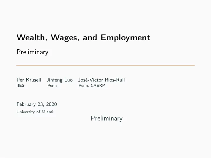
Wealth, Wages, and Employment

Preliminary

Per Krusell Jinfeng Luo José-Víctor Ríos-Rull

IIES Penn Penn, CAERP

February 23, 2020

University of Miami

Preliminary

Introduction

• We want a theory of the joint distribution of employment, wages,

and wealth, where

• Workers are risk averse, so only use self-insurance.
• Employment and wage risk are endogenous. (More concerned about

whether people work than about how long they work.)

• The economy aggregates into a modern economy (total wealth, labor

shares, consumption/investment ratios)

• Business cycles can be studied. In particular, we want to study

employment flows jointly with the other standard objects.

• The most sophisticated version compares well with fluctuations data.

1

Literature

• The steady state of this economy has as its core Aiyagari (1994)

meets Merz (1995), Andolfatto (1996) meets Moen (1997).

• Related Lise (2013), Hornstein, Krusell, and Violante (2011), Krusell, Mukoyama, and

Şahin (2010), Ravn and Sterk (2016, 2017), Den Haan, Rendahl, and Riegler (2015).

• Specially Eeckhout and Sepahsalari (2015), Chaumont and Shi (2017), Griffy (2017).
• Developing empirically sound versions of these ideas compels us to
• Add extreme value shocks as a form of accommodating quits and on

the job search as choices.

• Use new potent tools to address the study of fluctuations in

complicated economies Boppart, Krusell, and Mitman (2018)

2

What are the uses?

• The study of Business cycles including gross flows in and out of

employment, unemployment and outside the labor force

• Policy analysis where now risk, employment, wealth (including its

distribution) and wages are all responsive to policy.

• Get some insights into the extent of wage rigidity
• Life-Cycle versions of these ideas (under construction) will allow us

to assess how age dependent policies fare.

3

Today: Build the Theory Sequentially and discuss & Fluctua- tions from two types of shocks

• 1. No Quits: Exogenous Destruction, no Quits. Built on top of Growth
• Model. (GE version of Eeckhout and Sepahsalari (2015)): Not a lot of wage
• dispersion. Not a lot of job creation in expansions.
• 2. Add Endogenous Quits: Higher wage dispersion may arise to keep

workers longer (quits via extreme value shocks).

• 3. On the Job Search workers may get outside offers and take them.

(Similar but not the same as in Chaumont and Shi (2017)).

• 4. Outside of the Labor Force
• 5. All of the Above
• Employers commit both to either a wage or a wage schedule w(z)

that depends on the aggregate shock.

4

Key Findings

• If wages are fully fixed and committed (Drastic Wage rigidity)
• Both endogenous quits and on-the-job yield counter factual

procyclical unemployment and massive on the job search.

• Allowing the wage of an already formed job match to respond some

to aggregate shocks corrects this.

• Getting the right relative volatility of old and new wages and the

amount of job-to-job moves and quits provides a way to measure wage rigidity.

• With partial wage rigidity the model fares reasonably well with the
• data. A few things still to improve. (Excessive Job-to-JOB

transitions)

• Similar behavior to that in the Shimer/Hagedorn-Manowski debate.

Here we can try to move towards an accommodation of both points

• f view.

5

A Brief Look At Data

Relevant Properties in U.S. Data

Mean St Dev Relt Correl Perc to Output w Output Source Average Wage

• 0.44-0.84

0.24-0.37

Haefke et al. (2013)

New Wage

• 0.68-1.09

0.79-0.83

Haefke et al. (2013)

Unemployment 4-6 4.84

• 0.85

Campolmi&Gnocchi (2016)

Annual Quits (All) 10-40 4.20 0.85

Brown et al. (2017)

Annual Switches 25-35 4.62 0.70

Fujita&Nakajima (2016)

Consumption 75 0.78 0.86

NIPA

Investment 25 4.88 0.90

NIPA 6

Model 1: No (Endogenous) Quits Model

No (Endog) Quits: Precautionary Savings, Competitive Search

• Jobs are created by firms (plants). A plant with capital plus a worker

produce one (z) unit of the good (z is the aggregate state of the economy).

• Firms pay flow cost ¯

c to post a vacancy in market {w, θ}.

• Firms cannot change wage (or wage-schedule) afterwards.
• Think of a firm as a machine programmed to pay w or w(z)
• Plants (and their capital) are destroyed at rate δf .
• Workers quit exogenously at rate δh.
• Households differ in wealth and wages (if working) but not in
• productivity. There are no state contingent claims, nor borrowing.
• If employed, workers get w and save.
• If unemployed, workers produce b and search in some {w, θ}.
• General equilibrium: Workers own firms.

7

Order of Events of No Quits Model

• 1. Households enter the period with or without a job: {e, u}.
• 2. Production & Consumption: Employed produce z on the job.

Unemployed produce b at home. They choose savings.

• 3. Firm Destruction and Exogenous Quits :

Some Firms are destroyed (rate δf ) They cannot search this period. Some workers quit their jobs for exogenous reasons δh. Total job destruction is δ.

• 4. Search: Firms and the unemployed choose wage w and tightness θ.
• 5. Job Matching : M(V , U) : Some vacancies meet some unemployed

job searchers. A match becomes operational the following period. Job finding and job filling rates ψh(θ) = M(V ,U)

U

, ψf (θ) = M(V ,U)

V

.

8

No Quits Model: Household Problem

• Individual state: wealth and wage
• If employed: (a, w)
• If unemployed: (a)
• Problem of the employed: (Standard)

V e(a, w) = max

c,a′ u(c) + β [(1 − δ)V e(a′, w) + δV u(a)]

s.t. c + a′ = a(1 + r) + w, a ≥ 0

• Problem of the unemployed: Choose which wage to look for

V u(a) = max

c,a′,w u(c) + β

• ψh[θ(w)] V e(a′, w) + [1 − ψh[θ(w)]] V u(a′)
• s.t.

c + a′ = a(1 + r) + b, a ≥ 0 θ(w) is an equilibrium object

9

Firms Post vacancies: Choose wages & filling probabilities

• Value of wage-w job: uses constant k capital that depreciates at rate δk (Ω = k)

Ω(w) = z − kδk − w + 1 − δf 1 + r

• (1 − δh) Ω(w) + δh Ω
• Affine in w:

Ω(w) =

• z + k
• 1−δf

1+r δh − δk

− w

• 1+r

r+δf +δh−δf δh

Block Recursivity Applies (firms can be ignorant of Eq)

• Value of creating a firm: ψf [θ(w)] Ω(w) + [1 − ψf [θ(w)]] Ω
• Free entry condition requires that for all offered wages

¯ c + k = ψf [θ(w)] Ω(w) 1 + r + [1 − ψf [θ(w)]] Ω 1 + r ,

10

No (Endog) Quits Model: Stationary Equilibrium

• A stationary equilibrium is functions {V e, V u, Ω, g ′e, g ′u, w u, θ}, an

interest rate r, and a stationary distribution x over (a, w), s.t.

• 1. {V e, V u, g ′e, g ′u, w u} solve households’ problems, {Ω} solves the

firm’s problem.

• 2. Zero profit condition holds for active markets

¯ c + k = ψf [θ(w)] Ω(w) 1 + r + [1 − ψf [θ(w)]] k(1 − δ − δk) 1 + r , ∀w offered

• 3. An interest rate r clears the asset market
• a dx =
• Ω(w) dx.

11

Characterization of a worker’s decisions

• Standard Euler equation for savings

uc = β (1 + r) E {u′

c}

• A F.O.C for wage applicants

ψh[θ(w)] V e

w(a′, w) = ψh θ[θ(w)] θw(w) [V u(a′) − V e(a′, w)]

• Households with more wealth are able to insure better against

unemployment risk.

• As a result they apply for higher wage jobs and we have dispersion

12

How does the Model Work Worker’s wage application decision

0.5 1 1.5 2 2.5 3

Wealth

0.3 0.4 0.5 0.6 0.7 0.8 0.9 1

Wage

wapply(a)

13

How does the Model Work Worker’s saving decision

0.5 1 1.5 2 2.5 3

Wealth

0.3 0.4 0.5 0.6 0.7 0.8 0.9 1

Wage

lowest w apply(a) wapply(a) wstay(a)

14

Shortcomings of this model

• Silent on Quits and Job-To-Job Movements.
• Low Wage Dispersion
• Small differences in volatility between average and new wages
• Low unemployment volatility

15

Summary: No (Endog) Quits Model

• 1. Easy to Compute Steady-State with key Properties

i Risk-averse, only partially insured workers, endogenous unemployment ii Can be solved with aggregate shocks too iii Policy such as UI would both have insurance and incentive effects iv Wage dispersion small—wealth doesn’t matter too much v · · · so almost like two-agent model (employed, unemployed) of Pissarides despite curved utility and savings

• 2. In the following we examine the implications of a quitting choice

16

Endogenous Quits

Endogenous Quits: Beauty of Extreme Value Shocks

• Temporary Shocks to the utility of working or not working: Some

workers quit. (in addition to any intrinsic taste for leisure)

• Adds a (smoothed) quitting motive so that higher wage workers quit

less often: Firms may want to pay high wages to retain workers.

• Conditional on wealth, high wage workers quit less often.
• But Selection (correlation 1 between wage and wealth when hired) makes wealth trump

wages and those with higher wages have higher wealth which makes them quite more

• ften: Wage inequality collapses.
• We end up with a model with little wage dispersion but with endogenous quits that

respond to the cycle. 17

Quitting Model: Time-line

• 1. Workers enter period with or without a job: {e, u}.
• 2. Production occurs and consumption/saving choice ensues:
• 3. Exogenous job/firm destruction happens.
• 4. Quitting:
• e draw shocks {ǫe, ǫu} and make quitting decision.

Job losers cannot search this period.

• u draw shocks {ǫu

1, ǫu 2}. No decision but same expected means.

• 5. Search: New or Idle firms post vacancies. Choose {w, θ}.

Wealth is not observable. (Unlike Chaumont and Shi (2017)). Yet it is still Block Recursive

• 6. Matches occur

18

Quitting Model: Workers

• Workers receive i.i.d shocks {ǫe, ǫu} to the utility of working or not
• Value of the employed right before receiving those shocks:
• V e(a′, w) =
• max{V e(a′, w) + ǫe, V u(a′) + ǫu} dF ǫ

V e and V u are values after quitting decision as described before.

• If shocks are Type-I Extreme Value dbtn (Gumbel), then

V has a closed form and the ex-ante quitting probability q(a, w) is q(a, w) = 1 1 + eα[V e(a,w)−V u(a)] higher parameter α → lower chance of quitting.

• Hence higher wages imply longer job durations. Firms could pay

more to keep workers longer.

19

Quitting Model: Workers Problem

• Problem of the employed: just change

V e for V e V e(a, w) = max

c,a′ u(c) + β

• (1 − δ)

V e(a′, w) + δV u(a)

• s.t.

c + a′ = a(1 + r) + w, a ≥ 0

• Problem of the unemployed is like before except that there is an

added term E{max[ǫu

1, ǫu 2]}

So that there is no additional option value to a job.

20

Quitting Model: Value of the firm

• Ωj(w): Value with with j-tenured worker.

Free entry condition requires that for all offered wages ¯ c + k = 1 1 + r

• ψf [θ(w)] Ω0(w) + [1 − ψf [θ(w)]] Ω
• ,
• Probability of retaining a worker with tenure j at wage w is ℓj(w).

(One to one mapping between wealth and tenure)

ℓj(w) = 1 − qe[g e,j(a, w), w]

ge,j(a, w) savings rule of a j − tenured worker that was hired with wealth a

• Firm’s value

Ωj(w) = z − kδk − w + 1 − δf 1 + r {ℓj(w)Ωj+1(w) + [1 − ℓj(w)] Ω}

21

Quitting Model: Solving forward for the Value of the firm

Ω0(w) = (z − w − δkk) Q1(w) + (1 − δf − δk)k Q0(w), Q1(w) = 1 +

∞

• τ=0

1 − δf 1 + r 1+τ

τ

• i=0

ℓi(w)

• ,

Q0(w) =

∞

• τ=0

1 − δf 1 + r 1+τ [1 − ℓτ(w)] τ−1

• i=0

ℓi(w)

• .
• New equilibrium objects {Q0(w), Q1(w)}. Rest is unchanged.
• It is Block Recursive because wealth can be inferred from w and j.

(No need to index contracts by wealth (as in Chaumont and Shi (2017)) ).

22

Do we get More Wage Dispersion?

• This Model has the potential to get more wage dispersion
• Conditional on wealth higher wages lead to less quitting.
• So firms are willing to pay more to keep workers longer
• BUT we will see a problem

23

Value of the firm as wage varies: The Poor

• For the poorest, employment duration increases when wage goes up.
• Firms value is increasing in the wage

0.68 0.7 0.72 0.74 0.76 0.78 0.8

Wage

0.5 1 1.5

Firm Value: Omega

24

Value of the firm as wage varies: The Rich

• For the richest, employment duration increases but not fast enough.
• Firm value is slowly decreasing in wages (less than static profits).

0.75 0.8 0.85 0.9 0.95

Wage

0.2 0.4 0.6 0.8 1 1.2

Firm Value: Omega

25

Value of the firm: Accounting for Worker Selection

• Large drop from below to above equilibrium wages.
• In Equilibrium wage dispersion COLLAPSES due to selection.

0.65 0.7 0.75 0.8 0.85 0.9 0.95

Wage

0.5 1 1.5

Firm Value: Omega

• Related to the Diamond dispersion paradox but for very different

reasons.

26

Effect of Quitting: The Mechanism

• Two forces shape the dispersion of wages
• Agents quit less at higher paid jobs, which enlarge the spectrum of

wages that firms are willing to pay (for a given range of vacancy filling probability).

• However, by paying higher wages, firms attract workers with more

wealth.

• Wealthy people quit more often, shrink employment duration.
• In equilibrium, the wage gap is narrow (disappears?) and the effect
• f wealth dominates.

27

Value of the firm: Zero profit Job Finding Probability

• Increasing in Wage (up to Grid calculation): Unique wage.

0.03 0.04 0.05 0.06 0.07 0.08 0.09 0.1 0.11 0.12 0.02 0.04 0.06 0.08 0.1 0.12 0.14 28

Quitting Makes a Big Difference

• Job finding prob with Endo

0.03 0.04 0.05 0.06 0.07 0.08 0.09 0.1 0.11 0.12 0.1 0.2 0.3 0.4 0.5 0.6 29

Shortcommings

• Wage Dispersion Collapses
• Silent on Job-To-Job Movements.
• Unemployment Moves little (but more than the previous one) over

the cycle

• No difference in volatility between average and new wages
• Correlation 1 between Wealth when starting to work and wage

30

A Detour on How to Improve the Correlation Between Wealth and Wages

• Pose aiming (extreme value) shocks).
• This reduces the correlation between wages and wealth when first

hired.

• It will have many uses, we think.

31

On the Job Search

On the Job Search Model: Time-line

• 1. Workers enter period with or without a job: V e, V u.
• 2. Production & Consumption:
• 3. Exogenous Separation
• 4. Quitting? Searching? Neither?: Employed draw shocks (ǫe, ǫu, ǫs)

and make decision to quit, search, or neither. Those who quit become u′, those who search join the u, in case of finding a job become {e′, w ′} but in case of no job finding remain e′ with the same wage w and those who neither become e′ with w. V E(a′, w), is determined with respect to this stage.

• 5. Search : Potential firms decide whether to enter and if so, the

market (w) at which to post a vacancy; u and s assess the value of all wage applying options, receive match specific shocks {ǫw ′} and choose the wage level w ′ to apply. Those who successfully find jobs become e’, otherwise become u’. 6. V u(a′), {Ωj(w)} are determined with respect to this stage.

• 7. Match

32

On the Job Search: Household Probl

• After saving, the unemployed problem is
• V u(a′) =
• max

w ′

• ψh(w ′)V e(a′, w ′) + (1 − ψh(w ′))V u(a′) + ǫw ′

dF ǫ

• After saving, the employed choose whether to quit, search or neither
• V e(a′, w) =
• max{V e(a′, w) + ǫe, V u(a′) + ǫu, V s(a′, w) + ǫs}dF ǫ
• The value of searching is

V s(a′, w) =

• max

w ′

• ψh(w ′)V e(a′, w ′) + [1 − ψh(w ′)]V e(a′, w) + ǫw ′

dF ǫ

33

On the Job Search: Household choices

• The probabilities of quitting and of searching

q(a′, w) = 1 1 + exp(α[V e(a′, w) − V u(a′)]) + exp(α[V s(a′, w) − V u(a′) + µs]) , s(a′, w) = 1 1 + exp(α[V u(a′) − V s(a′, w)]) + exp(α[V e(a′, w) − V s(a′, w) − µs]) .

µs < 0 is the mode of the shock ǫs which reflects the search cost.

• Households solve

V e(a, w) = max

a′≥0 u[a(1 + r) + w − a′] + β

• δV u(a′) + (1 − δ)

V e(a′, w)

• V u(a) = max

c,a′≥0 u[a(1 + r) + b − a′] + β

V u(a′)

34

the Job Search Model: Value of the Firm

• The value of the firm is again given like in the Quitting Model

Ω0(w) = (z − w − δkk) Q1(w) + (1 − δ − δk)k Q0(w), Q1(w) = 1 +

∞

• τ=0

1 − δ 1 + r 1+τ

τ

• i=0

ℓi(w)

• ,

Q0(w) =

∞

• τ=0

1 − δ 1 + r 1+τ [1 − ℓτ(w)] τ−1

• i=0

ℓi(w)

• .
• Except that now the probability of keeping a worker after j periods is

ℓj(w) = 1 −

• h(w; a) q[g e,j(a, w), w] dxu(a)−
• h(w; a) s[w; g e,j(a, w)]
• ˆ

h[ w; g e,j(a, w), w]ξφh( w) d( w)

• dxu(a)

35

OJS Quitting Probabilities, Various wealths & Wage Density

0.3 0.4 0.5 0.6 0.7 0.8 0.9 1 1.1 0.1 0.2 0.3 0.4 0.5 0.6 0.7 0.8 0.9 0.005 0.01 0.015 0.02 0.025 0.03

• The rich pursue often other activities (leisure?)

36

Outside the Labor Force

Outside the Labor Force Model: Time-line

• 1. Workers enter period with or without a job: V e, V u.
• 2. In the beginning of the period non Workers get a shock to the utility
• f either searching or not searching.

They then choose whether to sit out and not search or to search. It is an extreme value shock.

Workers get a utility injection equal to the expected utility of the maximum of those two shocks to get no bias in the value of working versus not.

• 3. Production & Consumption:
• 4. Exogenous Separation
• 5. Quitting? Searching? Neither?:
• 6. Search

7.

• V u(a′), {Ωj(w)} are determined with respect to this stage.
• 8. Match

37

Various Economies with added Life Cycle (live 50 years)

• Provides a mechanism for having poor agents
• Right now we have Four Economies
• 1. Only Exogenous Quitting
• 2. Endogenous Quitting
• 3. Exogenous Quitting with On-the-job Search
• 4. Endogenous Quitting and On-the-job Search
• 5. ... and some agents do not want to work
• Today we will only look at the Economy with Endogenous quitting

and On-the-Job-Search (4)

38

Quantitative Analysis: Steady States

Parameter Values

Definition Value in Yearly Units r interest rate 3% K fixed capital required 3 δf firm destruction rate 2.88% δk capital maintenance rate 6.38% δh total worker quitting rate 8.56% cv job posting cost 0.03 y productivity on the job 1 b/w productivity at home 0.4 σ risk aversion 2 Matching function m = χuηv 1−η, non-OJS χ = 0.15, η = 0.62 m = χuηv 1−η, OJS χ = 0.3, η = 0.5

• We also explore a lower on the job search economy ()high value of

leisure economy b/w ∼ 0.75

39

Steady State Allocations in Yearly Units: Endog Quits & OJS

interest rate 0.030 avg consumption 0.651 avg wage 0.689 avg wealth 3.041 stock market value 2.953 avg labor income 0.654 consumption to wealth ratio 0.225 labor income to wealth ratio 0.215 quit ratio 0.090 unemployment rate 0.097 job losers 0.117 wage of newly hired unemp 0.677 std consumption 0.011 std wage 0.002 std wealth 3.606 mean-min consumption 2.051 mean-min wage 1.058 UE transition 0.125 total vacancy 0.578 avg unemp duration 0.773 avg emp duration 7.228 avg job duration 1.898 OJS move rate 0.395 40

Job Finding Probability Curves

0.56 0.58 0.6 0.62 0.64 0.66 0.68 0.7 0.72 0.74 0.76 0.05 0.1 0.15 0.2 0.25 41

Wage Distributions: Baseline

0.64 0.65 0.66 0.67 0.68 0.69 0.7 0.71 0.72 0.73 0.05 0.1 0.15 0.2 0.25 0.3 42

Wage Distributions: Comparing with lower OJS

0.64 0.66 0.68 0.7 0.72 0.74 0.05 0.1 0.15 0.2 0.25 0.3 0.64 0.66 0.68 0.7 0.72 0.74 0.05 0.1 0.15 0.2 0.25 0.3

43

Wage Applications of the Unemployed by Wealth

5 10 15 0.655 0.66 0.665 0.67 0.675 0.68 0.685

44

Wage Applications of U and w and densities of all

5 10 15 0.675 0.68 0.685 0.69 0.695 0.7 0.705 0.71 0.715 0.72 0.002 0.004 0.006 0.008 0.01 0.012 0.014 0.016

45

Aggregate Fluctuations

Introduce Aggregate Shocks

• We examine the model responses to two type of shocks
• 1. Productivity shocks zt: Output = EmpRate × (1 + zt)
• 2. Firm destruction shocks dt: Firm Destruction Rate = δf × (1 − dt)
• We introduce a wage peg assumption:
• To allow the wage of an already formed job match to respond to zt

shocks directly (by 50%) (but not to dt shocks)

• If wages were completely rigid there would be massive quits:

counterfactual.

46

1% Productivity Shock (ρ = .95) [IRF]

20 40 60 80 100 120 140

Period

0.1 0.2 0.3 0.4 0.5 0.6 0.7 0.8 0.9 1

Percent Deviations

New Wage Path

• Fig. 1: Wages

20 40 60 80 100 120

period

• 0.7
• 0.6
• 0.5
• 0.4
• 0.3
• 0.2
• 0.1

percent deviations

Unemployment Rate Path

• Fig. 2: Unemployment Rate
• Non-trivial response of wage and unemployment

47

1% Productivity Shock (ρ = .95) IRF

20 40 60 80 100 120 140

period

• 0.2

0.2 0.4 0.6 0.8 1 1.2 1.4

Percent Deviations

Quitting Rate Path

• Fig. 3: Quits

20 40 60 80 100 120 140

period

2 4 6 8 10 12

Percent Deviations

OJS Move Path

• Fig. 4: Job-to-job Moves
• Quits are mildly responsive to the shock
• While on-the-job moves are much more responsive: (perhaps too

much)

48

1% Delta Shock (ρ = .95)

20 40 60 80 100 120

Period

• 0.01

0.01 0.02 0.03 0.04 0.05 0.06

Percent Deviations

New Wage Path

• Fig. 5: Wages

20 40 60 80 100 120

period

• 0.25
• 0.2
• 0.15
• 0.1
• 0.05

percent deviations

Unemployment Rate Path

• Fig. 6: Unemployment Rate
• Again 1% delta shock = 0.36 base points
• Large response of wage and unemployment to the delta shock
• Note wage is not pegged to the delta shock

49

M4: 1% Delta Shock (ρ = .95)

20 40 60 80 100 120

period

• 0.05

0.05 0.1 0.15 0.2 0.25 0.3

Percent Deviations

Quitting Rate Path

• Fig. 7: Quits

20 40 60 80 100 120

period

• 0.2

0.2 0.4 0.6 0.8 1 1.2 1.4

Percent Deviations

OJS Move Path

• Fig. 8: Job-to-job Moves
• But too much volatility for job-to-job transitions relative to output

50

Summary, On-the-job Search and Quits

• Pro-cyclical average wages, new wages, and employment, quitting,

and job-to-job transitions

• Clear responses of new wages and employment
• Quitting mildly respnds to both shocks
• Job-to-job transitions move too much with both shocks

51

Assessing Performance in terms of standard hp-filtered 2nd moments

• 1st order data moments are from standard database: CPS, JOLTS,

LEHD and NIPA.

• 2nd order data moments are from Haefke, Sonntag, and Van Rens

(2013), Campolmi and Gnocchi (2016), Brown et al. (2017) and Fujita and Nakajima (2016).

52

Productivity Shock: Relative Volatility

• Only Productivity Shock: ρ = 0.95

Model Data Output 1 1 Average Wage 0.51 0.44-0.84 New Wage 0.95 0.68-1.09 Unemployment 0.35 4.84 Quits + OJS moves 8.94 4.2 OJS moves 10.66 4.62

Table 1: Standard Deviation Relative to Output: Only Productivity Shock

• Unemployment moves too little and Quits and OJS moves too much

53

Productivity Shock: Correlation

• Only Productivity Shock: ρ = 0.95

Model Data Output 1 1 Average Wage 1.00 0.24-0.37 New Wage 1.00 0.79-0.83 Unemployment

• 0.48
• 0.85

Quits + OJS moves 0.99 0.85 OJS moves 0.99 0.70

Table 2: Correlation with Contemprary Output: Only Productivity Shock

• Correlations are on the spot

54

Delta Shock: Relative Volatility

Model Data Output 1 1 Average Wage 0.09 0.44-0.84 New Wage 2.02 0.68-1.09 Unemployment 4.70 4.84 Quits + OJS moves 41.66 4.2 OJS moves 49.36 4.62

Table 3: Standard Deviation Relative to Output: Only Delta Shock

• Now Unemployment is good but moves are excessive
• Note that relative to output, productivity is very important so

employment cannot do that much, but this shock makes employment the

• nly culprit so it has to move a lot

55

Delta Shock: Correlation Only Delta Shock: ρ = 0.95

Model Data Output 1 1 Average Wage 0.13 0.24-0.37 New Wage 0.31 0.79-0.83 Unemployment

• 0.99
• 0.85

Quits + OJS moves 0.40 0.85 OJS moves 0.42 0.70

Table 4: Correlation with Contemprary Output: Only Delta Shock

56

Both Shocks: Relative Volatility Very correlated (.95)

Model Data Output 1 1 Average Wage 0.49 0.44-0.84 New Wage 1.38 0.68-1.09 Unemployment 3.02 4.84 Quits + OJS moves 25.77 4.2 OJS moves 30.53 4.62

Table 5: Standard Deviation Relative to Output: Both Shocks

• Relative Std of shocks: each shock contributes roughly equal to
• utput volatility

57

Both Shocks: Correlation 0.95

Model Data Output 1 1 Average Wage 0.77 0.24-0.37 New Wage 0.50 0.79-0.83 Unemployment

• 0.37
• 0.85

Quits + OJS moves 0.28 0.85 OJS moves 0.29 0.70

Table 6: Correlation with Contemprary Output: Both Shocks

• Relative Std of shocks: each shock contributes roughly equal to
• utput volatility

58

Both Shocks: Relative Volatility Uncorrelated

Model Data Output 1 1 Average Wage 0.40 0.44-0.84 New Wage 1.35 0.68-1.09 Unemployment 2.59 4.84 Quits + OJS moves 23.98 4.2 OJS moves 28.45 4.62

Table 7: Standard Deviation Relative to Output: Both Shocks

• Relative Std of shocks: each shock contributes roughly equal to
• utput volatility

59

Both Shocks: Correlation Uncorrelated

Model Data Output 1 1 Average Wage 0.82 0.24-0.37 New Wage 0.62 0.79-0.83 Unemployment

• 0.61
• 0.85

Quits + OJS moves 0.47 0.85 OJS moves 0.48 0.70

Table 8: Correlation with Contemprary Output: Both Shocks

60

Clumsy Experiments & Extensions

Several Experiments/Extensions

• Now we move to some experiments/extensions to illustrate/evaluate

the business cycle performance of the model

• We look at the following
• 1. An Exogenous quitting Economy with higher b that illuminates the

Shimer/Hagedorn-Manowski debate.

• 2. An Economy with on the job search and quitting with lower ξ (the

intensity of on-the-job search) such that J2J is 29% rather than 40% per year.

• 3. An Economy with on the job search and quitting and higher wage

pegs (from 0.5 to 0.95).

• 4. An Economy with on the job search and quitting and different

matching functions for UE and EE moves.

61

1- High-b Economy: (Without quits or OJS only TFP)

Low-b High-b Mean Std Corr Mean Std Corr Output 1 1 1 1 1 1 Avg Wage 0.70 0.51 1.00 0.74 0.33 0.84 New Wage 0.70 0.73 0.99 0.74 0.38 0.84 Unemp Rate 12.6% 0.28

• 0.55

22.2% 0.97

• 0.86

Table 9: The High-b Benchmark Economy: M1

• Much higher unemployment volatility due to higher b
• higher wages and thus lower firm profits in s-s, amplifying the move
• f job finding probability due to aggregate shocks
• We are moving towards an economy with two types of b and agents
• ccasionally move across types. V: (Not done yet)
• such that most quits are due to type stwitchers

62

2- Baseline: and Low Ave J-2-J 1% Productivity Shock (ρ = .95)

20 40 60 80 100

Period

0.1 0.2 0.3 0.4 0.5 0.6 0.7 0.8 0.9

Percent Deviations Wage Path average wage of all the employed average wage of the newly hired from the unemployed

• Fig. 9: Wages

20 40 60 80 100 120

period

• 1.2
• 1
• 0.8
• 0.6
• 0.4
• 0.2

percent deviations Unemployment Rate Path

• Fig. 10: Unemployment Rate
• Similar Wage Responses
• 70% more unemployment volatility which mainly comes from more

responsive quits

63

2- Baseline and Low Ave J-2-J 1% Productivity Shock (ρ = .95)

20 40 60 80 100 120

period

• 1
• 0.5

0.5 1 1.5 2 2.5 3

Percent Deviations Quitting Rate Path

• Fig. 11: Quits

20 40 60 80 100 120

period

2 4 6 8 10 12 14

Percent Deviations OJS Move Path

• Fig. 12: Job-to-job Moves
• More quitting
• Similar (excessive) J-2-J transitions

64

2- Baseline: and Low Ave J-2-J 1% Delta Shock (ρ = .95)

20 40 60 80 100 120

Period

• 0.01

0.01 0.02 0.03 0.04 0.05 0.06

Percent Deviations Wage Path average wage of all the employed average wage of the newly hired from the unemployed

• Fig. 13: Wages

20 40 60 80 100 120

period

• 0.3
• 0.25
• 0.2
• 0.15
• 0.1
• 0.05

0.05

percent deviations Unemployment Rate Path

• Fig. 14: Unemployment Rate
• Similar Wage Response
• 16% more unemployment response
• Note wage is not pegged to the delta shock

65

2- Baseline: with Low Ave J-2-J 1% Delta Shock (ρ = .95)

20 40 60 80 100 120

period

• 0.2
• 0.1

0.1 0.2 0.3 0.4 0.5 0.6

Percent Deviations Quitting Rate Path

• Fig. 15: Quits

20 40 60 80 100 120

period

0.5 1 1.5

Percent Deviations OJS Move Path

• Fig. 16: Job-to-job Moves
• More Quits
• Similar (excessive) volatility for job-to-job transitions

66

2- Baseline: with Low Ave J-2-J: Business Cycle Statistics

• Two ways to aggregate shocks

shock corr = 0.95 shock corr = 0 Std corr Std corr

• utput

1.00 1.00 1.00 1.00 avg wage 0.41 0.93 0.41 0.90 new wage 1.69 0.76 1.38 0.52 unemployment 2.59

• 0.73

2.80

• 0.63

quits + j2j movers 29.85 0.77 26.72 0.38 J2J movers 36.30 0.79 32.51 0.41

• Not too successful in reducing volatility of quits and J2J movers.
• Need to look for alternatives.

67

3- Baseline with Higher Wage Peg (.8): 1% TFP (ρ = .95)

20 40 60 80 100 120

period

• 1
• 0.5

0.5 1 1.5 2 2.5 3

Percent Deviations

Quitting Rate Path

Wage Peg = 0.5 Wage Peg = 0.8

• Fig. 17: Quits

20 40 60 80 100 120

period

• 0.1

0.1 0.2 0.3 0.4 0.5 0.6 0.7 0.8 0.9

OJS Search Path

Wage Peg = 0.5 Wage Peg = 0.8

• Fig. 18: OJS Searchers
• Higher wage peg lowers the reponse of on-the-job search and quit.
• Workers find it less so attractive to move/quit as existing wages now

comove more with the productivity shock

68

3- Baseline with Higher Wage Peg (.8): 1% TFP (ρ = .95)

20 40 60 80 100 120

period

2 4 6 8 10 12 14

OJS Move Path

Wage Peg = 0.5 Wage Peg = 0.8

• Fig. 19: Job-to-job transitions

20 40 60 80 100 120

period

• 1.2
• 1
• 0.8
• 0.6
• 0.4
• 0.2

0.2

Percent Deviations

Unemployment Rate Path

Wage Peg = 0.5 Wage Peg = 0.8

• Fig. 20: Unemployment
• Job-to-job transition rate also lowers: from 12% to 9%. This is from
• less search on the job (see Fig 18)
• less improvement of job finding rate due to smaller s-s firm profits
• Also less persistence of the unemployment response (less turnover).
• However j2j transition rate still moves much more than

unemployment

69

3- Baseline with Higher Wage Peg (.8): 1% TFP (ρ = .95)

Wage Peg = 0.5 Wage Peg = 0.8 Mean Std Corr Mean Std Corr Output 1 1 1 1 1 1 Avg Wage 0.690 0.51 1.00 0.690 0.76 0.99 New Wage 0.689 0.95 1.00 0.689 1.04 0.99 Unemp Rate 10.6% 0.35

• 0.48

10.6% 0.42

• 0.64

Quits+J2J moves 38.4% 8.94 0.99 38.4% 6.65

• 0.99

J2J moves 29.2% 10.66 0.99 29.2% 8.50

• 0.99

Table 10: M4 Compare Wage Pegs: Productivity Shock (ρ = 0.95)

• Lowers j2j transition volatility while raises unemployment volatility
• Still, j2j transition volatility is much higher than unemployment

volatility

• In the next several pages we take a closer look at this problem

70

A Fundamental Tension

• In all of the above exercises we find that the volatility of j2j

transition rate is a magnitude larger than unemployment rate

• However, in the data unemployment rate is as volatile as (or even

more volatile than) the j2j transition rate.

• Difficult to deliver this in the model from aggregate shocks affecting

jobs at all wage levels

• The percentage changes of firm value, vacancy filling probability and

job finding probability are similar at all wage levels

• Thus as a stock, the response of unemployment would thus be a

magnitude smaller than the j2j transition rate (a flow)

71

A Fundamental Tension: the Fix

• Two potential fixes
• Make the value of the firm at high wages be more volatile ⇒ hard

since high-wage matches feature low profits

• Make the job finding probability of the employed less responsive to

the same percentage change in the firm value ⇒ curvature in the matching function controls this

• Motivated by this, we will allow η in the matching function

m = χuηv 1−η to be low in UE moves but high in EE moves

• ψh(w) = χ(

χ ψf (w))

1−η η

⇒ ln ψh(w) = 1

η ln χ − 1−η η

ln ψf (w)

• Higher η ⇒ smaller response of ψh(w) to ψf (w)
• Lower ηu from 0.5 to 0.35 and raise ηe from 0.5 to 0.75

72

4- Baseline plus Different Matching Functions for UE & EE

ηe = ηu = 0.5 ηe = 0.75, ηu = 0.35 Mean Std Corr Mean Std Corr Output 1 1 1 1 1 1.00 Avg Wage 0.690 0.51 1.00 0.688 0.53 1.00 New Wage 0.689 0.95 1.00 0.654 0.92 1.00 Unemp Rate 10.6% 0.35

• 0.48

7.7% 0.78

• 0.84

Quits+J2J moves 38.4% 8.94 0.99 34.9% 1.42 1.00 J2J moves 29.2% 10.66 0.99 26.9% 1.98 1.00

Table 11: Baseline with Different Matching Functions: TFP Shocks

• It greatly reduces the volatility gap between unemployment and j2j

transitions

• But they both show insufficient volatility compared to output, in

response to the productivity shock

73

4- Baseline plus Different Matching Functions for UE & EE

ηe = ηu = 0.5 ηe = 0.75, ηu = 0.35 Mean Std Corr Mean Std Corr Output 1 1 1 1 1 1 Avg Wage 0.690 0.15 0.13 0.688 0.45 0.47 New Wage 0.689 2.02 0.31 0.654 2.40 0.73 Unemp Rate 10.6% 4.55

• 0.99

7.7% 9.37

• 0.99

Quits+J2J moves 38.4% 42.41 0.40 34.9% 11.65 0.70 J2J moves 29.2% 49.40 0.42 26.9% 15.55 0.70

Table 12: M4 Different Matching Functions: Delta Shock (ρ = 0.95)

• It reduces the volatility gap between unemployment and j2j

transitions

• Unemployment is much more volatile compared to output in

response to the delta shock, because the delta shock only affects total output through employment

74

4- Baseline plus Different Matching Functions for UE & EE

• Two ways to aggregate shocks

shock corr = 0 shock corr = 0.95 Std corr Std corr

• utput

1.00 1.00 1.00 1.00 avg wage 0.48 0.91 0.41 0.94 new wage 1.20 0.80 1.34 0.96 unemployment 3.70

• 0.52

3.30

• 0.91

quits + j2j movers 4.88 0.60 5.01 0.94 J2J movers 6.50 0.62 6.68 0.96

Table 13: M4 Both Shocks (ηe = 0.75, ηu = 0.35, ρ = 0.95)

• By allowing for two types of shocks, and different matching

functions for UE and EE moves, the model delivers a pretty good match to the data

75

Conclusions I

• Develop tools to get a joint theory of wages, employment and wealth

that marry the two main branches of modern macro:

• 1. Aiyagari models (output, consumption, investment, interest rates)
• 2. Labor search models with job creation, turnover, wage

determination, flows between employment, unemployment and

• utside the labor force.
• 3. Add tools from Empirical Micro to generate quits
• Useful for business cycle analysis: We are getting procyclical
• Quits
• Employment
• Investment and Consumption
• Wages
• On the Job Search are quite important to understand employment

volatility and give us a good sense of how (upward) flexible wages are.

76

Conclusions II

• Exciting set of continuation projects:
• 1. Incorporate the movements outside of the labor force.
• 2. Endogenous Search intensity on the part of firms
• 3. Aiming Shocks to soften correlation between wages and wealth
• 4. Efficiency Wages: Endogenous Productivity (firms use different

technologies with different costs of idleness)

• 5. Move towards more sophisticated household structures (more life

cycle movements, multiperson households).

77

Firms choose Search Intensity

• The number of vacancies posted is chosen by firms
• Easy to implement
• Slightly Different steady state

78

Free entry with variable recruiting intensity

• Let υ(c) be a technology to post vacancies where c is the cost paid.
• Then the free entry condition requires that for all offered wages

0 = max

c

• υ(c) ψf [θ(w)] Ω(w)

1 + r +

• 1 − υ(c) ψf [θ(w)]
• k(1 − δk)

1 + r − c − k

• ,
• With FOC given by

vc(c)

• ψf [θ(w)]

Ω(w) 1 + r − k(1 − δk) 1 + r

• = 1,

79

How to make it consistent with the current steady state

• If v(c) = υ1c2

2

+ υ2 c, we have (υ1 c + υ2)

• ψf [θ(w)]

Ω(w) 1 + r − k(1 − δk) 1 + r

• = 1,
• By Choosing υ so that for the numbers that have now

υ1c2 2 + υ2 c

• ψf [θ(w)] Ω(w)

1 + r +

• 1 − υ1c2

2 − υ2 c

• ψf [θ(w)] k(1 − δk)

1 + r

• = c + k,
• Solving for {υ1, υ2} that satisfy both equations given our choice of c

we are done

80

References

Aiyagari, S. Rao. 1994. “Uninsured Idiosyncratic Risk and Aggregate Saving.” Quarterly Journal of Economics 109 (3):659–684. Andolfatto, D. 1996. “Business Cycles and Labor-Market Search.” American Economic Review 86(1):112–132. Boppart, Timo, Per Krusell, and Kurt Mitman. 2018. “Exploiting MIT shocks in heterogeneous-agent economies: the impulse response as a numerical derivative.” Journal of Economic Dynamics and Control 89 (C):68–92. URL https://ideas.repec.org/a/eee/dyncon/v89y2018icp68-92.html. Brown, Alessio JG, Britta Kohlbrecher, Christian Merkl, and Dennis J Snower. 2017. “The effects of productivity and benefits on unemployment: Breaking the link.” Tech. rep., GLO Discussion Paper. Campolmi, Alessia and Stefano Gnocchi. 2016. “Labor market participation, unemployment and monetary policy.” Journal of Monetary Economics 79:17–29. Chaumont, Gaston and Shouyong Shi. 2017. “Wealth Accumulation, On the Job Search and Inequality.” Https://ideas.repec.org/p/red/sed017/128.html. Den Haan, Wouter, Pontus Rendahl, and Markus Riegler. 2015. “Unemployment (Fears) and Deflationary Spirals.” CEPR Discussion Papers 10814, C.E.P.R. Discussion Papers. URL https://ideas.repec.org/p/cpr/ceprdp/10814.html. Eeckhout, Jan and Alireza Sepahsalari. 2015. “Unemployment Risk and the Distribution of Assets.” Unpublished Manuscript, UCL. Fujita, Shigeru and Makoto Nakajima. 2016. “Worker flows and job flows: A quantitative investigation.” Review of Economic Dynamics 22:1–20. Griffy, Benjamin. 2017. “Borrowing Constraints, Search, and Life-Cycle Inequality.” Unpublished Manuscript, UC Santa Barbara. Haefke, Christian, Marcus Sonntag, and Thijs Van Rens. 2013. “Wage rigidity and job creation.” Journal of Monetary Economics 60 (8):887–899. Hornstein, Andreas, Per Krusell, and Gianluca Violante. 2011. “Frictional Wage Dispersion in Search Models: A Quantitative Assessment.” American Economic Review 101 (7):2873–2898. Krusell, Per, Toshihiko Mukoyama, and Ayşegul Şahin. 2010. “Labour-Market Matching with Precautionary Savings and Aggregate Fluctuations.” Review of Economic Studies 77 (4):1477–1507. URL https://ideas.repec.org/a/oup/restud/v77y2010i4p1477-1507.html. Lise, Jeremy. 2013. “On-the-Job Search and Precautionary Savings.” The Review of Economic Studies 80 (3):1086–1113. URL +http://dx.doi.org/10.1093/restud/rds042. Merz, M. 1995. “Search in the Labor Market and the Real Business Cycle.” Journal of Monetary Economics 36 (2):269–300. Moen, Espen R. 1997. “Competitive Search Equilibrium.” Journal of Political Economy 105 (2):385–411. Ravn, Morten O. and Vincent Sterk. 2016. “Macroeconomic Fluctuations with HANK & SAM: An Analytical

81

Steady-States

m1 m2 m3 m4 m4 (low xi) β 0.975 0.972 0.975 0.976 0.976 interest rate 0.030 0.030 0.030 0.030 0.030 avg consumption 0.686 0.682 0.691 0.684 0.680 avg wage 0.707 0.719 0.696 0.689 0.690 avg wealth 2.789 2.763 2.361 3.041 2.919 stock market value 2.971 2.692 3.065 2.953 2.931 avg labor income 0.659 0.655 0.668 0.654 0.652 consumption to wealth ratio 0.246 0.247 0.293 0.225 0.233 labor income to wealth ratio 0.236 0.237 0.283 0.215 0.223 quit ratio 0.090 0.088 0.090 0.090 0.092 unemployment rate 0.129 0.165 0.076 0.097 0.106 job losers 0.117 0.115 0.117 0.117 0.119 wage of newly hired unemployed 0.707 0.719 0.656 0.677 0.689 std consumption 0.013 0.010 0.011 0.011 0.011 std wage 0.000 0.000 0.003 0.002 0.001 std wealth 2.989 2.715 2.624 3.606 3.677 mean-min consumption 2.057 2.045 2.072 2.051 2.039 mean-min wage 1.012 1.001 1.094 1.058 1.042 UE transition 0.121 0.114 0.128 0.125 0.126 total vacancy 0.544 0.308 0.704 0.578 0.707 avg unemp duration 1.062 1.449 0.589 0.773 0.745 avg emp duration 7.228 7.335 7.228 7.228 7.131 OJS move rate 0.000 0.000 0.420 0.395 0.292 avg job duration 7.228 7.335 1.814 1.898 2.342

Wage Distributions

0.6 0.65 0.7 0.75 0.1 0.2 0.3 0.4 0.5 0.6 0.7 0.8 0.9 1 0.6 0.65 0.7 0.75 0.1 0.2 0.3 0.4 0.5 0.6 0.7 0.8 0.9 1 0.6 0.65 0.7 0.75 0.1 0.2 0.3 0.4 0.5 0.6 0.7 0.8 0.9 1 0.6 0.65 0.7 0.75 0.1 0.2 0.3 0.4 0.5 0.6 0.7 0.8 0.9 1 0.6 0.65 0.7 0.75 0.1 0.2 0.3 0.4 0.5 0.6 0.7 0.8 0.9 1

Derive the Idle Value

• Value of an idle firm is

Ω0 = −δkk + 1 − δf 1 + r

• −cv + ψf Ω + (1 − ψf )Ω0
• Free entry

k = 1 1 + r

• −cv + ψf Ω + (1 − ψf )Ω0
• Newly entered firms do not receive the destruction shock immediately
• Vacancy posting cost is paid immediately before searching
• Combine the above

Ω0 = (1 − δf − δk)k