Weak coupling -> standard Cooper pairs (BCS type) Weak - PowerPoint PPT Presentation
Germn Sierra Instituto de Fsica Terica CSIC-UAM, Madrid, Spain Work in progress done in collaboration with J. Links and S. Y. Zhao (Univ. Queensland, Australia) and M. Ibaez (IFT, Madrid) Talked presented at the INSTANTS Conference at
Germán Sierra Instituto de Física Teórica CSIC-UAM, Madrid, Spain Work in progress done in collaboration with J. Links and S. Y. Zhao (Univ. Queensland, Australia) and M. Ibañez (IFT, Madrid) Talked presented at the INSTANTS Conference at the Galileo Galilei Institute, Firenze, September 2008.
- Recent interest in p-wave superconductivity is motivated by its applications to He3 films, superconductors as Sr2RuO4, superfluids of fermi cold atoms in optical traps, etc. - p+ip pairing symmetry in the BCS model gives rise to the pfaffian state, which is closely related to the Moore and Read state for the Fractional Quantum Hall state for the filling fraction 5/2. When considering the vortices in the BCS model one gets non abelians anyons similar to those of the Moore-Read model (Green-Read 2000). Thus the p+ip superconductors allows for Topological Quantum Computation, although non universal. - So far the studies of the BCS model with p+ip symmetry are based on a mean-field analysis using the BdG Hamiltonian. The corresponding phase diagram contains three regions:
• Weak coupling -> “standard” Cooper pairs (BCS type) • Weak pairing -> “Moore Read” pairs • Strong pairing -> localized Cooper pairs (BEC type) The weak and strong pairing regions are separated by a second order phase transition where the gap vanishes. The mean field wave function also experiences a “topological phase transition” across these two regions (Volovik). The boundary between the weak pairing and the weak coupling regions has not been well characterized. It is thus of great interest to have an exactly solvable BCS model with p+ip symmetry to analyze in detail the nature of the Moore-Read Pfaffian state and the different phases boundaries of the model.
This model is the so called “reduced” BCS model with p+ip wave symmetry and it is analogous to the reduced BCS model with s-wave symmetry. The latter model was solved by Richardson in 1963 and it is closely related to the Gaudin spin Hamiltonians. The Richardson model was extensively used to study ultrasmall superconducting grains made of Al in the 1990s. The integrability of the Richardson-Gaudin models can be proved using the standard Quantum Inverse Scattering Methods. These are the methods that we apply to the p+ip model.
Outline - The pfaffian state in the BCS model - Mean-field approach to the p + i p model - Exact Bethe ansatz solution - Numerical solution of the BAEs - Thermodynamic limit: electrostatic analogy. Connection between the mean-field and the exact solution - Puzzles in the weak pairing region
The BCS state (Proyected BCS state) for p-wave N � � � � BCS � exp 1 * c � r * c � r � � * * g r k c r � 0 � PBCS � g r k c r 0 � � � k k k k 2 r r � � � � k k * c r Operator that creates a polarised electron with momenta k k g r Wave function of the Cooper pair in momentum space k The proyected state has 2N electrons with wave function � ( r 1 , K , r 2 N ) = A � ( r 1 � r 2 ) � ( r 3 � r 4 ) K � ( r 2 N � 1 � r [ ] r r r r r r r r 2 N ) r r � ( r k � r � r ) = g ( k )exp( i r ) r k This wave function is a pfaffian = sqrt(determinant) Moore-Read corresponds to the long distance/small momenta behaviour: r r � ( r ) � 1/( x + i y ), r r r � � , g ( k ) � 1/( k x + ik y ), k � 0
The reduced BCS Hamiltonian with p+ip wave symmetry reads: r 2 k � G * c r * c � * c � � � H = 2 m c r ( k x + i k y )( k � x � i k � y ) c r k � c r r r k k k k k � 4 m r r r k k � k ' To be compared with the s-wave symmetry (Richardson model) r 2 k � � c r * * * H = 2 m c r c r � G c � c � k � , � c r r r k , � k , � k , � k , � k � , � r r r k , � k � k ' In the standard mean-field approximation: � ( k x � ik y ) c � k c r � = r k r k r � � 2 k � G 2 m � µ * c r � � ( ) H = c r � ( k x � i k y ) c � k � c r k � + h . c . � � r k k 2 2 m r � � k x > 0, k y k Which can be diagonalized by a Bogoliubov transformation
µ The gap and chemical potential are solution of the eqs (m=1) � r 2 k 2 = 1 � r r 2 + G 2 � µ 2 � ( ) k k k x � 0, k y 1 2 = 2 N � L + 1 � µ r r 2 + G 2 � µ 2 � ( ) k k k x � 0, k y L is the number of energy levels and N is the number of pairs The thermodynamic limit is defined by L � � , N � � , G � 0 x = N Such that are constant g = G L , L ( filling factor ) The solution of the gap and chemical potential eqs yield µ = µ ( g , x ), � = � ( g , x )
The mean field wave function: N � � � � BCS � exp 1 * c � r * c � r � � * * g r k c r � 0 � PBCS � g r k c r 0 � � � k k k k 2 r r � � � � k k r r 2 + µ r ) = v r = E ( k ) � k k g ( k ( ) � * u r k x + ik y k r r r 2 2 � µ 2 � where ( ) 2 is the energy of the quasiparticles E ( k ) = k k + µ The behaviour as k -> 0 depends crucially on the sign of µ < 0 � g ( r ) � k x � i k y , � ( r ) � e � r / r 0 : Strong pairing phase k r µ > 0 � g ( r , � ( r 1 1 k ) � r ) � x + i y : Weak pairing phase k x + i k y At there is a second order phase transition (Read-Green line) µ = 0 r r E ( k ) � k � 0 but there is also a topological transition
Topological nature of the weak-strong transition (Volovik) Momentum space Wave function � r g ( r � k ) � 0 k � � 0 µ > 0 � r � k � 0 µ < 0 0 0 � Winding number of the map S 2 � S 2 : + 1 µ > 0 ( weak pairing ) � 0 µ < 0 ( strong pairing ) �
Solution of the gap and chemical potential equations Parameterize the dispersion relation as r r r r r 2 = 2 2 � µ 2 � 2 � a 2 � b ( ) ( ) ( ) E ( k ) = k k k k + The parameters a and b have a meaning in the electrostatic solution of the exact model (see later) µ > � 2 Weak coupling a , b = � 0 ± i � 0 x > x MR 4 � � x MR = 1 � 1 µ = � 2 Moore � Re ad line a = b = � µ � � 4 g � � 0 < µ < � 2 Weak pairing a < b < 0 x RG < x < x MR 4 � � x RG = 1 2 1 � 1 Re ad � Green line a < b = 0 µ = 0 � � g � � Strong pairing a < b < 0 µ < 0 x < x RG
Phase diagram of the p + ip wave model
Duality between weak and strong pairing phase Given two points in the phase diagram ( g , x I ) � weak pairing phase ( µ > 0) ( g , x II ) � strong pairing phase ( µ < 0) If x I + x II = 1 � 1 g � E I = E II , � I = � II , µ I = � µ II The Read-Green line is selfdual The Moore-Read line is dual to the “empty” state x = 0 (in particular the GS energy on this line is zero) This duality also appears in the exact solution and plays an important role.
Recall the Hamiltonian: r 2 k � G * c r * c � * c � � � H = 2 m c r ( k x + i k y )( k � x � i k � y ) c r k � c r r r k k k k k � 4 m r r r k k � k ' r 2 / m 2 = Setting z r k k * = k x � ik y * c � Define the hard core boson operators: * b r r c r r k k k k Then the Hamiltonian can be brought into the form 2 N r * b r � � H = z r k � G z r k z r k � b r k k k � r r k x � 0, k y k � k � And can be solved using the Quantum Inverse Scattering Method starting from the XXZ R-matrix and taking a quasi-classical limit
H � = E � The Schroedinger equation: is solved exactly by the states (m=1) N k x � ik * c � � � r * C ( y m ) 0 , C ( y ) = 2 � y c r � = r k k k m = 1 k x � 0, k y y m where the “rapidities” satisfy the Bethe ansatz eqs � G � 1 � L + 2 N � 1 L N 1/2 1 � � ( m = 1, K , N ) = 0 � 2 + y m y m � z k y m � y j k = 1 j � m N � E = (1 + G ) y m The total energy is m = 1 2 lim G � 0 y m = z k For G � 0 � y m : real or complex Complex solutions always appear in conjugate pairs
Roots of the p + i p model (numerical solution with L=12,N=6, x=1/2) Im y m Re y m
Roots in the complex y-plane (p + i p model) g
Roots for the exactly solvable s-wave model g
x = N L , N � � , G � 0, with , g = GL finite L � y m Let us assume that the roots form an arc in the complex plane r ( y ) with a density 2 � ( � ) � = z k The energies form another arc with density � The BAEs become � � y � q 0 � ( � ) r ( y � ) � � d � y � P dy � y �� y = 0, y � � � � q 0 = 1 2 G � L 2 + N � � N = dy r ( y ), E = dy y r ( y ) � � There is a analytic solution of these equations which agree with the mean-field solution to leading order in L and N
Structure of the arcs formed by the roots y
The equation of the complex arc can be determined and compared with the numerical results: Example with x = 1/2 and g = 1.99 (weak coupling region)
x � x MR = 1 � 1 The Moore-Read line y m � 0 � m � g N k x � i k y * c � r Recall � � * r C ( y m ) 0 , C ( y ) = c r � = 2 � y k k k m = 1 k x � 0, k y N 1 * c � r MR state � * � C (0) = c r C (0) 0 , � � = k k k x + i k y k x � 0, k y m = 1
Recommend
More recommend
Explore More Topics
Stay informed with curated content and fresh updates.
