WaveScalar Good old days 2 Good old days ended in Nov. 2002 - PowerPoint PPT Presentation
WaveScalar Good old days 2 Good old days ended in Nov. 2002 Complexity Clock scaling Area scaling 3 Chip MultiProcessors Low complexity Scalable Fast 4 CMP Problems Hard to program Not practical to scale
WaveScalar �
Good old days 2
Good old days ended in Nov. 2002 Complexity Clock scaling Area scaling 3
Chip MultiProcessors Low complexity Scalable Fast 4
CMP Problems Hard to program Not practical to scale There only ~8 threads Inflexible allocation Tile = allocation Thread parallelism only 5
What is WaveScalar? WaveScalar is a new, scalable, highly parallel processor architecture Not a CMP Different algorithm for executing programs Different hardware organization 6
WaveScalar Outline Dataflow execution model Hardware design Evaluation Exploiting dataflow features Beyond WaveScalar: Future work 7
Execution Models: Von Neumann Von Neumann (CMP) Program counter Centralized Sequential 8
Execution Model: Dataflow Not a new idea [Dennis, ISCA’75] Programs are dataflow graphs 2 2 Instructions fire when data arrives Instructions act independently + + All ready instructions can fire at once Massive parallelism 4 Where are the dataflow machines? 9
Von Neumann example Mul t1 ← i, j Mul t2 ← i, i A[j + i*i] = i; Add t3 ← A, t1 Add t4 ← j, t2 b = A[i*j]; Add t5 ← A, t4 Store (t5) ← i Load b ← (t3) 10
Dataflow example i A j * * A[j + i*i] = i; + + b = A[i*j]; Load + Store b 11
Dataflow example i A j * * A[j + i*i] = i; + + b = A[i*j]; Load + Store b 12
Dataflow example i A j * * A[j + i*i] = i; + + b = A[i*j]; Load + Store b 13
Dataflow example i A j * * A[j + i*i] = i; + + b = A[i*j]; Load + Store b 14
Dataflow example i A j * * A[j + i*i] = i; + + b = A[i*j]; Load + Store b 15
Dataflow example i A j * * A[j + i*i] = i; + + b = A[i*j]; Load + Store b 16
Dataflow’s Achilles’ heel No ordering for memory operations No imperative languages (C, C++, Java) Designers relied on functional languages instead To be useful, WaveScalar must solve the dataflow memory ordering problem 17
WaveScalar’s solution i A j Order memory operations * * Just enough + + ordering Preserve parallelism Load + Store b 18
Wave-ordered memory Load 2 3 4 Compiler annotates Store 3 4 ? memory operations Sequence # Successor 4 5 6 Store Load 4 7 8 Predecessor Load 5 6 8 Send memory requests in any order Hardware reconstructs the Store ? 8 9 correct order 19
Wave-ordering Example Store buffer Load 2 3 4 2 3 4 Store 3 4 ? 3 4 ? 4 5 6 Store Load 4 7 8 Load 5 6 8 4 7 8 ? 8 9 Store ? 8 9 20
Wave-ordered Memory Wave s are loop-free sections of the control flow graph Each dynamic wave has a wave number Each value carries its wave number Total ordering Ordering between waves “linked list” ordering within waves [MICRO’03] 21
Wave-ordered Memory Annotations summarize the CFG Expressing parallelism Reorder consecutive operations Alternative solution: token passing [Beck, JPDC’91] 1/2 the parallelism 22
WaveScalar’s execution model Dataflow execution Von Neumann-style memory Coarse-grain threads Light-weight synchronization 23
WaveScalar Outline Execution model Hardware design Scalable Low-complexity Flexible Evaluation Exploiting dataflow features Beyond WaveScalar: Future work 24
Executing WaveScalar i A j Ideally * * One ALU per instruction + Direct communication + Practically Fewer ALUs Load + Reuse them Store b 25
WaveScalar processor architecture Array of processing elements (PEs) Dynamic instruction placement/eviction 26
Processing Element Simple, small 0.5M transistors 5-stage pipeline Holds 64 instructions 27
PEs in a Pod 28
Domain 29
Cluster 30
WaveScalar Processor 31
WaveScalar Processor Long distance communication Dynamic routing Grid-based network 32K instructions ~400mm 2 90nm 22FO4 (1Ghz) 32
WaveScalar processor architecture Thread Low complexity Thread Scalable Thread Thread Flexible parallelism Thread Flexible allocation Thread 33
Demo 34
Previous dataflow architectures Many, many previous dataflow machines [Dennis, ISCA’75] TTDA [Arvind, 1980] Sigma-1 [Shimada, ISCA’83] Manchester [Gurd, CACM’85] Epsilon [Grafe, ISCA’89] EM-4 [Sakai, ISCA’89] Monsoon [Papadopoulos, ISCA’90] *T [Nikhil, ISCA’92] 35
Previous dataflow architectures Many, many previous dataflow machines [Dennis, ISCA’75] Modern TTDA [Arvind, 1980] technology Sigma-1 [Shimada, ISCA’83] Manchester [Gurd, CACM’85] WaveScalar Epsilon [Grafe, ISCA’89] architecture EM-4 [Sakai, ISCA’89] Monsoon [Papadopoulos, ISCA’90] *T [Nikhil, ISCA’92] 36
WaveScalar Outline Execution model Hardware design Evaluation Map WaveScalar’s design space Scalability CMP comparison Exploiting dataflow features Beyond WaveScalar: Future work 37
Performance Methodology Cycle-level simulator Workloads SpecINT + SpecFP Splash2 Mediabench Binary translator from Alpha -> WaveScalar Alpha Instructions per Cycle (AIPC) Synthesizable Verilog model 38
WaveScalar’s design space Many, many parameters # of clusters, domains, PEs, instructions/PE, etc. Very large design space No intuition about good designs How to find good designs? Search by hand Complete, systematic search 39
WaveScalar’s design space Constrain the design space Synthesizable RTL model -> Area model Fix cycle time (22FO4) and area budget (400mm 2 ) Apply some “common sense” rules Focus on area-critical parameters There are 201 reasonable WaveScalar designs Simulate them all 40
WaveScalar’s design space [ISCA’06] 41
Pareto Optimal Designs [ISCA’06] 42
WaveScalar is Scalable 7x apart in area and performance 43
Area efficiency Performance per silicon: IPC/mm 2 WaveScalar 1-4 clusters: 0.07 16 clusters: 0.05 Pentium 4: 0.001-0.013 Alpha 21264: 0.008 Niagara (8-way CMP): 0.01 44
WaveScalar Outline Execution model Hardware design Evaluation Exploiting dataflow features Unordered memory Mix-and-match parallelism Beyond WaveScalar: Future work 45
The Unordered Memory Interface Wave-ordered memory is restrictive Circumvent it Manage (lack-of) ordering explicitly Load_Unordered Store_Unordered Both interfaces co-exist happily Combine with fine-grain threads 10s of instructions 46
Exploiting Unordered Memory Fine-grain intermingling struct { int x,y; } Pair; foo(Pair *p, int *a, int *b) { Pair r; *a = 0; r.x = p->x; r.y = p->y; return *b; } 47
Exploiting Unordered Memory Ordered Fine-grain intermingling St *a, 0 <0,1,2> Unordered Mem_nop_ack <1,2,3> struct { int x,y; } Pair; Ld p->y Ld p->x foo(Pair *p, int St r.x St r.y *a, int *b) { Pair r; + *a = 0; r.x = p->x; Mem_nop_ack <2,3,4> r.y = p->y; return *b; Ld *b <3,4,5> } 48
Exploiting Unordered Memory Ordered Fine-grain intermingling St *a, 0 <0,1,2> Unordered Mem_nop_ack <1,2,3> struct { int x,y; } Pair; Ld p->y Ld p->x foo(Pair *p, int St r.x St r.y *a, int *b) { Pair r; + *a = 0; r.x = p->x; Mem_nop_ack <2,3,4> r.y = p->y; return *b; Ld *b <3,4,5> } 49
Exploiting Unordered Memory Ordered Fine-grain intermingling St *a, 0 <0,1,2> Unordered Mem_nop_ack <1,2,3> struct { int x,y; } Pair; Ld p->y Ld p->x foo(Pair *p, int St r.x St r.y *a, int *b) { Pair r; + *a = 0; r.x = p->x; Mem_nop_ack <2,3,4> r.y = p->y; return *b; Ld *b <3,4,5> } 50
Exploiting Unordered Memory Ordered Fine-grain intermingling St *a, 0 <0,1,2> Unordered Mem_nop_ack <1,2,3> struct { int x,y; } Pair; Ld p->y Ld p->x foo(Pair *p, int St r.x St r.y *a, int *b) { Pair r; + *a = 0; r.x = p->x; Mem_nop_ack <2,3,4> r.y = p->y; return *b; Ld *b <3,4,5> } 51
Exploiting Unordered Memory Ordered Fine-grain intermingling St *a, 0 <0,1,2> Unordered Mem_nop_ack <1,2,3> struct { int x,y; } Pair; Ld p->y Ld p->x foo(Pair *p, int St r.x St r.y *a, int *b) { Pair r; + *a = 0; r.x = p->x; Mem_nop_ack <2,3,4> r.y = p->y; return *b; Ld *b <3,4,5> } 52
Exploiting Unordered Memory Ordered Fine-grain intermingling St *a, 0 <0,1,2> Unordered Mem_nop_ack <1,2,3> struct { int x,y; } Pair; Ld p->y Ld p->x foo(Pair *p, int St r.x St r.y *a, int *b) { Pair r; + *a = 0; r.x = p->x; Mem_nop_ack <2,3,4> r.y = p->y; return *b; Ld *b <3,4,5> } 53
Recommend
More recommend
Explore More Topics
Stay informed with curated content and fresh updates.
