Water in South Florida Agriculture Julie Harrington, Yuki - PowerPoint PPT Presentation

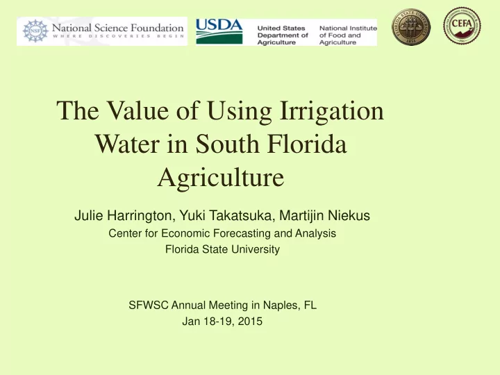
The Value of Using Irrigation Water in South Florida Agriculture Julie Harrington, Yuki Takatsuka, Martijin Niekus Center for Economic Forecasting and Analysis Florida State University SFWSC Annual Meeting in Naples, FL Jan 18-19, 2015

Basic Framework 1 Introduction 2 Economic Analysis of Water Use – Model Assumptions E and Production Function Water Penalty Function – Analysis and Results 3 Water Penalty Function – Spatial Analysis 4 5 Summary 2

Project Director: Julie Harrington, Ph.D. Center for Economic Forecasting and Analysis, The Florida State University Water, Sustainability and Climate for South Florida – Category 2 Collaborative: Robust decision-making for south Florida water resources by ecosystem service valuation, hydro-economic optimization, and conflict resolution modeling Objective: Approach: • To develop adaptive water management schemes that • The South Florida Water Sustainability Project are capable of sustaining important social-ecological comprises about 7 task or working group areas. The interactions, while accounting for uncertainty in larger- value of water will be analyzed in its direct use (e.g., scale stressors associated with climate change, sea level sector outputs), in socio-ecologic use (e.g., water rise, and economic settings. storage and flood control), and in non-use (e.g., sustainability). • To develop a regional-scale hydro-economic model that • The first task involves the economic analysis of urban is capable of optimizing the resilience of water supplies and agricultural water use. In addition, the project for the built & natural systems while also accounting for team will examine the potential risks and economic the broad-sector value of water use and water quality impacts of salt water intrusion from SLR. improvements. Impact: Participating local, state, and federal agencies responsible for managing the region’s water resources, among other stakeholders, will benefit from these broad-sector analyses of adaptive schemes that explicitly incorporate uncertainty estimates of potential outcomes.

Introduction The Florida Department of Environmental Protection (FDEP) and South Florida Water Management District (SFWMD) conveyed that traditional sources of fresh groundwater would have difficulty meeting all of the additional demands by 2030 (FLDEP, 2013 and SFWMD, 2012). What is the economic loss (water penalty) if water is under shortage?

SFWMD REGION % County NO AREA NO County Area Kissimmee Basin (KB) 1 1 Glades 0.60 1 2 Highlands 0.75 1 3 Okeechobee 0.75 1 4 Orange 0.32 1 5 Osceola 0.73 1 6 Polk 0.24 Lower East Coast (LEC) 2 7 Broward 1.00 2 8 Collier 0.09 2 9 Hendry 0.48 2 10 Miami-Dade 1.00 2 11 Monroe 0.56 2 12 Palm Beach 1.00 Lower West Coast (LWC) 3 13 Charlotte 0.35 3 14 Collier 0.91 3 15 Glades 0.40 3 16 Hendry 0.52 3 17 Lee 1.00 3 18 Monroe 0.44 Upper East Coast (UEC) 4 19 Martin 1.00 4 20 Okeechobee 0.13 4 21 St Lucie 1.00

Economic Variables and Input Data Used in the Water Penalty in SFWMD CV SWC GWC SWC/ ($ millions) EMPC (acre-ft) (acre-ft) (SWC+GWC) RICL FR CL YEAR $ 4,406 27,176 1,860,824 805,354 0.70 0.84 0.94 1,169,025 2000 2005 $ 4,471 25,180 1,445,617 596,459 0.71 0.83 0.88 1,056,914 2010 $ 3,234 20,698 1,072,932 548,780 0.66 0.79 0.73 973,252 CV = the value of farm cropland products sold in million dollars , which his adjusted according to the inflation rate based on the producer price index cropland in 2010 (PPI 2010=100). EMPC = employment in cropland SWC = surface water usage in cropland in acre-foot per year (acre-ft) GWC = ground water usage in cropland in acre-foot per year (acre-ft) RICL =the ratio of irrigated cropland out of the cultivated cropland FR =the ratio of fertilized cropland out of the cultivated cropland CL = the size of cropland (acres)

SFWMD and Associated Subdistricts REGI ON REGIO CV ($ SWC/(SWC+ NO N YEAR millions) EMPC SWC (acre-ft) GWC (acre-ft) GWC) RICL RF CL 1 KB 2000 $ 617 3,045 57,231 159,615 0.26 0.77 0.92 186,968 2005 $ 649 2,724 66,124 133,319 0.33 0.77 0.83 175,570 2010 $ 446 2,917 93,818 101,124 0.48 0.75 0.70 157,693 2 LEC 2000 $ 2,441 15,837 1,209,633 261,927 0.82 0.88 0.97 603,375 2005 $ 2,533 14,321 973,746 195,076 0.83 0.86 0.90 564,272 2010 $ 1,864 12,014 598,084 161,094 0.79 0.77 0.72 544,306 3 LWC 2000 $ 929 6,937 237,193 311,545 0.43 0.90 0.96 206,981 2005 $ 886 6,953 186,026 220,900 0.46 0.88 0.88 190,902 2010 $ 650 4,915 273,623 271,108 0.50 0.85 0.71 174,264 4 UEC 2000 $ 419 1,357 356,767 72,266 0.83 0.80 0.92 171,701 2005 $ 402 1,182 219,721 47,164 0.82 0.80 0.90 126,170 2010 $ 274 852 107,407 15,454 0.87 0.78 0.81 96,990

Assumptions Used in Cobb-Douglas Production Function The level of surface water use changes from SWCo (the current/original level) to SWCn (the new or future level). If all other variables are held constant, then the production (value of crop sold) level would change from CVo to CVn. The difference of the production level (d CV) is: d CV i,t = CVn i,t - CVo i,t

Empirical Framework: Cobb-Douglas Production Function and Results c SWC i,t d GWC i,t e RICL i,t f FR i,t g YEAR i,t h . CV i,t = a EMPC i,t which can be rewritten as + d ln SWC i, t + e ln GWC i, t + f ln RICL i, t ln CV i, t = ln a + c ln EMPC i, t + g ln FR i, t + h ln YEAR i, t . Standard Coefficients Error t Stat P-value -0.497 0.395 -1.26 0.22 ln a 0.550 ** 0.040 13.65 0.00 ln EMPC 0.078 ** 0.032 2.42 0.02 ln SWC 0.136 ** 0.044 3.07 0.00 ln GWC 0.692 ** 0.325 2.13 0.04 ln RICL 1.440 ** 0.593 2.43 0.02 ln FR 0.290 ** 0.133 2.18 0.04 ln YEAR 0.928 R Square 0.917 Adjusted R Square 0.000 P-value 45 Observations ** siginificant at the 0.05 level

Marginal Benefit of Water Using Cobb-Douglas Production Function 0.550 SWC i,t 0.078 GWC i,t 0.136 RICL i,t 0.692 FR i,t 1.440 YEAR i,t 0.290 . CV i,t = a i,t EMPC i,t The difference of the production level (d CV) is: d CV i,t = CVn i,t - CVo i,t = (a i,t EMPC i,t 0.290 ) – 0.550 SWCn , i,t 0.078 GWC i,t 0.136 RICL i,t 0.692 FR i,t 1.440 YEAR i,t 0.550 SWCo i,t 0.078 GWC i,t 0.136 RICL i,t 0.692 FR i,t 1.440 YEAR i,t 0.290 ) (a i,t EMPC i,t

Marginal Benefit of Water Using Cobb-Douglas Production Function 0.550 SWC i,t 0.078 GWC i,t 0.136 RICL i,t 0.692 FR i,t 1.440 YEAR i,t 0.290 . CV i,t = a i,t EMPC i,t The marginal benefit (MB) of water? Producer’s value marginal product (VMP) for surface water VMPS i,t =∂ CV i,t /∂ SWC i,t 0.550 SWC i,t (0.078-1) = a i,t (0.0078) EMPC i,t 0.136 RICL i,t 0.692 FR i,t 1.440 YEAR i,t 0.290 GWC i,t

Marginal Benefit (MB) of Water in SFWMD Regions Surface Ground Water Water 2000 2005 2010 2000 2005 2010 KB $ 845 $ 770 $ 372 $ 527 $ 665 $ 601 LEC $ 158 $ 204 $ 244 $ 1,272 $ 1,772 $ 1,579 LWC $ 307 $ 373 $ 186 $ 407 $ 547 $ 327 UEC $ 92 $ 144 $ 200 $ 791 $ 1,164 $ 2,423 SFWMD $ 186 $ 243 $ 236 $ 747 $ 1,023 $ 804 ($ / acre-ft per year)

Water Penalty Function (1) : Cost When farmers decide upon the irrigation water level, we assume that their objective is to maximize their profits by adjusting the amount of water use. Thus, water can be optimally used and efficiently allocated in cropland when farmers choose the amount of irrigation. Under this condition, producer’s profit is maximized, which interprets that the marginal benefit (MB) of the use of irrigation water is equal to the marginal cost (MC) of supply of irrigation water (Young, 2005 and Dudu and Chumi, 2008). MC i,t = MB i,t = VMPS i,t . If the surface water levels are changed from the current level (SWCo) to the new level (SWCn), then the cost difference (d COST) associated by the change in water use (SWn-SWo) can be calculated by the following: d COST i,t =( MC i,t ) ( SWCn i,t -SWCo i,t ).

Water Penalty Function (2) Water penalty is profit loss when the amount of irrigation water is changed: = CV i,t – COST i,t Profit = d CV i,t – d COST i,t PENALTY i,t PENALTY i,t = (CVn i,t - CVo i,t ) – (MC i,t ) ( SWCn i,t -SWCo i,t )

Water Penalty Function (3) Water penalty is profit loss when the amount of irrigation water is changed: PENALTY i,t = d CV i,t – d COST i,t = (CVn i,t - CVo i,t ) – (MC i,t ) ( SWCn i,t -SWCo i,t ) 0.078 – (0.078 b1 i,t ) SWCo i,t (0.078-1) PENALTY i,t = b1 i,t SWCn i,t (d SWC i,t ) - CVo i,t , 0.550 GWC i,t 0.136 RICL i,t 0.692 where b1 i,t = a i,t EMPC i, t 1.440 YEAR i,t 0.290 , and FR i,t d SWC i,t = SWCn i,t -SWCo i,t

Water Penalty Results for SFWMD Regions