VISGRAF LAB WEBINAR 2020-09-23 The leopard never changes its - PowerPoint PPT Presentation
VISGRAF LAB WEBINAR 2020-09-23 The leopard never changes its spots: realistic pigmentation pattern formation by coupling tissue growth with reaction-diffusion Marcelo de Gomensoro Malheiros - FURG Henrique Fensterseifer - UFRGS Marcelo
VISGRAF LAB WEBINAR 2020-09-23 The leopard never changes its spots: realistic pigmentation pattern formation by coupling tissue growth with reaction-diffusion Marcelo de Gomensoro Malheiros - FURG Henrique Fensterseifer - UFRGS Marcelo Walter - UFRGS
OVERVIEW ● Pigment formation ● Tissue growth ● Pattern enlargement ● Results ● Conclusions sample code at mgmalheiros.github.io 2
RESEARCH GOAL ● We aim to realistically reproduce animal patterns – but we also want to get insights into the underlying biological processes – therefore, we look for a plausible explanation for pigmentation pattern formation – for that, we have explored the expressiveness of combining simple mechanisms – we have found that reaction-diffusion and tissue growth both play crucial roles 3
PIGMENT FORMATION ● Reaction-Diffusion (RD) ● Implementation ● Exploratory approach
REACTION-DIFFUSION » OVERVIEW ● Pioneering work of Alan Turing ● Models autocatalytic chemical reactions ∂ a ● PDEs involving two reagents A and B: 2 a ∂ t = 16 − ab + D a ∇ – a and b are local concentrations ∂ b – there are reaction and diffusion parts 2 b ∂ t = ab − b − 12 + D b ∇ – diffusion depends on nearby concentrations – D a and D b are the diffusion rates 5
REACTION-DIFFUSION » DISCRETIZATION ● RD is typically solved by numerical methods ● Forward Euler integration is simple and fast ● The domain is a square lattice: Δ a =( 16 − ab + D a ∇ 2 a )Δ t – a and b are now two matrices – ∇ 2 a and ∇ 2 b are the Laplacian operators, Δ b =( ab − b − 12 + D b ∇ 2 b )Δ t implemented by finite differences – we use a 9-point stencil, with the given weights 1 4 1 around a center cell 4 -20 4 / 6 1 4 1 6
REACTION-DIFFUSION » SIMULATION ● First, define the initial values for a and b ● Given Δt , loop until a final time is reached a next = a +Δ a ● At each iteration: – compute Laplacians for all matrix elements b next = b +Δ b – evaluate Δa and Δb a = clip ( a next ,L a ,U a ) – calculate a next and b next – limit a next by lower bound L a and upper bound U a b = clip ( b next , L b ,U b ) – limit b next by lower bound L b and upper bound U b 7
REACTION-DIFFUSION » INITIAL CONDITIONS ● Reaction-diffusion is sensitive to initial values ● However, pattern formation is also robust : – small perturbations yield small pattern changes – a fixed set of parameters induces the same resulting pattern structure, despite the randomness ● For most experiments we use: – a initial = 4 – b initial = 4 + uniform random noise in [0, 1] 8
REACTION-DIFFUSION » BOUNDARY CONDITIONS ● We employ two types of boundaries: – toroidal wrapping → matrix borders wrap around – no-flux boundary → matrix borders have their concentrations extended outward 9
REACTION-DIFFUSION » VISUALIZATION ● The Turing model exhibits cross kinetics, that is, A and B are completely out of phase ● For display: – we typically map either the a or b matrices a to a perceptually-uniform color map – some experiments also use a simple linear- interpolated color map – no further alteration b 10
EXPLORATORY APPROACH » PARAMETERS ● We have explored the parameter space of the original model, and then proposed extensions to improve expressibility and usage: – let D a = r s and D b = s – r is the ratio between diffusion rates → structure – s expresses the overall pattern scale – previously L b = 0 , but we found that positive values also alter the pattern structure – setting U a and U b also changes the dynamics 11
EXPLORATORY APPROACH » PARAMETER MAPS ratio (x) × U a (y) ratio (x) × L b (y) 12
TISSUE GROWTH ● Static and growing domains ● Matrix expansion ● Effect of growth
STATIC DOMAIN ● Normal Turing patterns present a space-filling behavior ● Patterns tend to create equispaced features : – spots – stripes or labyrinths – a mix of both ● The average distance between features is called the pattern wavelength 14
GROWING DOMAIN » TWO PREVIOUS APPROACHES ● #1 Add continuous growth term to PDEs: – simulation still runs over a square lattice ● #2 A point-based cellular model, following the biologic analogy: – diffusion occurs only among nearby cells – cells divide and push others ● The drawback is being expensive: – needs collision mechanics – needs repeated Nearest Neighbor Search 15
GROWING DOMAIN » A NOVEL APPROACH ● Here we propose matrix expansion : – we approximate uniform growth by randomly selecting matrix elements and duplicating them – this is performed once for each row → yields a new column – then it is performed once for each column → yields a new row ● The domain is always a regular matrix: – on average, cell divisions are uniformly spread – we define a growth rate during simulation 16
EFFECT OF GROWTH » INITIAL STATE 17
EFFECT OF GROWTH » ONLY GROWTH, NO DIFFUSION 18
EFFECT OF GROWTH » GROWTH AND REACTION-DIFFUSION 19
EFFECT OF GROWTH » GROWTH AND SATURATED REACTION-DIFFUSION 20
PATTERN ENLARGEMENT ● Problem ● Continuous reinforcement ● Effect of growth
PROBLEM ● How to maintain the overall pattern appearance during growth? – cell division adds noise! – large constant areas need to expand – borders must be kept well-defined: sharp, not blurry ● Reaction-diffusion does not have these properties, but a similar model can achieve this photo by m_bos (Pixabay licence) 22
CONTINUOUS REINFORCEMENT » OVERVIEW ● Models an autocatalytic reaction ● Has a dual effect: smoothing and ∂ c ∂ t =γ( t − w − c )( t − c )( t + w −c )+ D c ∇ 2 c maintenance ● PDE involving reagent C: – c is the local concentration – there are reaction and diffusion parts – diffusion depends on nearby concentrations – D c is the diffusion rate 23
CONTINUOUS REINFORCEMENT » GROWTH AND REINFORCEMENT 24
RESULTS ● Impact of initial state ● Simulated biologic patterns
RESULTS » PREPATTERN ● The initial state of the simulation is called a prepattern ● We employed two types of prepatterns: – random initial concentration – local random production ● Simulations have two or more phases ● The resulting concentrations of a phase are directly fed into the next phase 26
RESULTS » RANDOM INITIAL CONCENTRATION ● Prepattern: – reagent A starts constant – reagent B starts constant plus a small random variation ● The first phase usually develops into spots ● Many works state the ubiquity of spots in early embryonic development 27
RESULTS » RETICULATE WHIPRAY 28 photo by Brian Gratwicke (Flickr, CC BY 2.0)
RESULTS » RETICULATE WHIPRAY 29 photo by Brian Gratwicke (Flickr, CC BY 2.0)
RESULTS » HONEYCOMB WHIPRAY 30 photo by the authors
RESULTS » HONEYCOMB WHIPRAY 31 photo by the authors
RESULTS » YELLOW-BANDED POISON DART FROG photo by Adrian Pingstone (Wikimedia Commons, public domain) 32
RESULTS » YELLOW-BANDED POISON DART FROG photo by Adrian Pingstone (Wikimedia Commons, public domain) 33
RESULTS » LOCAL RANDOM PRODUCTION ● Prepattern: – reagent A starts constant – reagent B starts constant – B is produced in small random amounts, along the dorsal spine ● The first phase usually develops into straight stripes ● Growth noise disrupts the stripes in very interesting ways 34
RESULTS » THIRTEEN-LINED GROUND SQUIRREL photo by Mnmazur (Wikimedia Commons, public domain) 35
RESULTS » THIRTEEN-LINED GROUND SQUIRREL photo by Mnmazur (Wikimedia Commons, public domain) 36
RESULTS » LEOPARD photo by Derek Keats (Flickr, CC BY 2.0) 37
RESULTS » LEOPARD photo by Derek Keats (Flickr, CC BY 2.0) 38
RESULTS » LEOPARD ● With a single set of parameters: – stripes develop into spatially-organized spots – due to growth, spots split into rosettes – limited growth in the dorsal spine produces deformed rosettes – shorter growth phases provide continuous variation of rosettes on other parts of the body 39 photo by Derek Keats (Flickr, CC BY 2.0)
RESULTS » LEOPARD ● Important insights: – the residual pattern before growth provides the brown spots – pheomelanin (reddish pigment) and eumelanin (black pigment) are induced by the same process ● 3D rendering: – simple mapping from final concentrations to pigmentation, using a specialized fur shader – visual complexity arises from fur orientation and self-shading 40
CONCLUSIONS ● Contributions ● Future work
CONCLUSIONS » CONTRIBUTIONS ● Tissue growth can be successfully approximated by matrix expansions ● The extended RD model provides great expressiveness and more intuitive controls ● A continuous reinforcement equation is demonstrated ● We emphasize the importance of the careful definition of the initial state ● We have generated a few unprecedented 2D patterns matching real species 42
Recommend
More recommend
Explore More Topics
Stay informed with curated content and fresh updates.
