VARMA versus VAR for Macroeconomic Forecasting George - PowerPoint PPT Presentation
VARMA versus VAR for Macroeconomic Forecasting 1 VARMA versus VAR for Macroeconomic Forecasting George Athanasopoulos Department of Econometrics and Business Statistics Monash University Farshid Vahid School of Economics Australian National
VARMA versus VAR for Macroeconomic Forecasting 1 VARMA versus VAR for Macroeconomic Forecasting George Athanasopoulos Department of Econometrics and Business Statistics Monash University Farshid Vahid School of Economics Australian National University
VARMA versus VAR for Macroeconomic Forecasting Introduction 2 Outline Introduction 1 Canonical SCM 2 Forecast performance 3 Example 4 Simulation 5 Summary of findings and future research 6
VARMA versus VAR for Macroeconomic Forecasting Introduction 3 VAR models dominate Why VARMA? More parsimonious representation Closed with respect to linear transformations
VARMA versus VAR for Macroeconomic Forecasting Introduction 3 VAR models dominate Why VARMA? More parsimonious representation Closed with respect to linear transformations Difficult to Identify “If univariate ARIMA modelling is difficult then VARMA modelling is even more difficult - some might say impossible!” - Chatfield
VARMA versus VAR for Macroeconomic Forecasting Introduction 3 VAR models dominate Why VARMA? More parsimonious representation Closed with respect to linear transformations Difficult to Identify “If univariate ARIMA modelling is difficult then VARMA modelling is even more difficult - some might say impossible!” - Chatfield Identification Problem � y 1 , t � φ 11 � � y 1 , t − 1 � ε 1 , t � θ 11 � � ε 1 , t − 1 � � � � φ 12 θ 12 = + − y 2 , t φ 21 φ 22 y 2 , t − 1 ε 2 , t θ 21 θ 22 ε 2 , t − 1 y 2 , t = ε 2 , t ⇒ y 2 , t − 1 = ε 2 , t − 1 ⇒ ( φ 12 , θ 12 ) - SCM framework: Tiao & Tsay (1989) completed by Athanasopoulos & Vahid (2006) - Echelon form: Hannan & Kavalieris (1984); Poskitt (1992); L¨ utkepohl & Poskitt (1996), Athanasopoulos, Poskitt & Vahid (2007)
VARMA versus VAR for Macroeconomic Forecasting Introduction 4 VAR models dominate Why VARMA? More parsimonious representation Closed with respect to linear transformations Difficult to Identify “If univariate ARIMA modelling is difficult then VARMA modelling is even more difficult - some might say impossible!” - Chatfield Identification Problem � � � � � � � � � � � � y 1 , t φ 11 φ 12 y 1 , t − 1 ε 1 , t θ 11 θ 12 ε 1 , t − 1 = + − 0 0 0 0 y 2 , t y 2 , t − 1 ε 2 , t ε 2 , t − 1
VARMA versus VAR for Macroeconomic Forecasting Introduction 4 VAR models dominate Why VARMA? More parsimonious representation Closed with respect to linear transformations Difficult to Identify “If univariate ARIMA modelling is difficult then VARMA modelling is even more difficult - some might say impossible!” - Chatfield Identification Problem � � � � � � � � � � � � y 1 , t φ 11 φ 12 y 1 , t − 1 ε 1 , t θ 11 θ 12 ε 1 , t − 1 = + − 0 0 0 0 y 2 , t y 2 , t − 1 ε 2 , t ε 2 , t − 1 y 2 , t = ε 2 , t ⇒ y 2 , t − 1 = ε 2 , t − 1
VARMA versus VAR for Macroeconomic Forecasting Introduction 4 VAR models dominate Why VARMA? More parsimonious representation Closed with respect to linear transformations Difficult to Identify “If univariate ARIMA modelling is difficult then VARMA modelling is even more difficult - some might say impossible!” - Chatfield Identification Problem � � � � � � � � � � � � y 1 , t φ 11 φ 12 y 1 , t − 1 ε 1 , t θ 11 θ 12 ε 1 , t − 1 = + − 0 0 0 0 y 2 , t y 2 , t − 1 ε 2 , t ε 2 , t − 1 y 2 , t = ε 2 , t ⇒ y 2 , t − 1 = ε 2 , t − 1 ⇒ ( φ 12 , θ 12 )
VARMA versus VAR for Macroeconomic Forecasting Introduction 4 VAR models dominate Why VARMA? More parsimonious representation Closed with respect to linear transformations Difficult to Identify “If univariate ARIMA modelling is difficult then VARMA modelling is even more difficult - some might say impossible!” - Chatfield Identification Problem � � � � � � � � � � � � y 1 , t φ 11 φ 12 y 1 , t − 1 ε 1 , t θ 11 θ 12 ε 1 , t − 1 = + − 0 0 0 0 y 2 , t y 2 , t − 1 ε 2 , t ε 2 , t − 1 y 2 , t = ε 2 , t ⇒ y 2 , t − 1 = ε 2 , t − 1 ⇒ ( φ 12 , θ 12 ) - SCM framework: Tiao & Tsay (1989) completed by Athanasopoulos & Vahid (2006) - Echelon form: Hannan & Kavalieris (1984); Poskitt (1992); L¨ utkepohl & Poskitt (1996), Athanasopoulos, Poskitt & Vahid (2007)
VARMA versus VAR for Macroeconomic Forecasting Canonical SCM 5 Outline Introduction 1 Canonical SCM 2 Forecast performance 3 Example 4 Simulation 5 Summary of findings and future research 6
VARMA versus VAR for Macroeconomic Forecasting Canonical SCM 6 Definition of a SCM: For a given K -dimensional VARMA ( p , q ) y t = Φ 1 y t − 1 + . . . + Φ p y t − p + η t − Θ 1 η t − 1 − . . . − Θ q η t − q (1)
VARMA versus VAR for Macroeconomic Forecasting Canonical SCM 6 Definition of a SCM: For a given K -dimensional VARMA ( p , q ) y t = Φ 1 y t − 1 + . . . + Φ p y t − p + η t − Θ 1 η t − 1 − . . . − Θ q η t − q (1) ′ y t ∼ SCM ( p r , q r ) z r , t = α r α r ′ Φ p r � = 0 T where 0 ≤ p r ≤ p if α r satisfies α r ′ Φ l = 0 T for l = p r + 1 , ..., p α r ′ Θ q r � = 0 T where 0 ≤ q r ≤ q α r ′ Θ l = 0 T for l = q r + 1 , ..., q
VARMA versus VAR for Macroeconomic Forecasting Canonical SCM 6 Definition of a SCM: For a given K -dimensional VARMA ( p , q ) y t = Φ 1 y t − 1 + . . . + Φ p y t − p + η t − Θ 1 η t − 1 − . . . − Θ q η t − q (1) ′ y t ∼ SCM ( p r , q r ) z r , t = α r α r ′ Φ p r � = 0 T where 0 ≤ p r ≤ p if α r satisfies α r ′ Φ l = 0 T for l = p r + 1 , ..., p α r ′ Θ q r � = 0 T where 0 ≤ q r ≤ q α r ′ Θ l = 0 T for l = q r + 1 , ..., q SCM Methodology: Find K-linearly independent vectors A = ( α 1 , . . . , α K ) ′ which transform (1) into Ay t = Φ ∗ 1 y t − 1 + . . . + Φ ∗ p y t − p + ε t − Θ ∗ 1 ε t − 1 − . . . − Θ ∗ (2) q ε t − q where Φ ∗ i = AΦ i , ε t = A η t and Θ ∗ i = AΘ i A − 1
VARMA versus VAR for Macroeconomic Forecasting Canonical SCM 6 Definition of a SCM: For a given K -dimensional VARMA ( p , q ) y t = Φ 1 y t − 1 + . . . + Φ p y t − p + η t − Θ 1 η t − 1 − . . . − Θ q η t − q (1) ′ y t ∼ SCM ( p r , q r ) z r , t = α r α r ′ Φ p r � = 0 T where 0 ≤ p r ≤ p if α r satisfies α r ′ Φ l = 0 T for l = p r + 1 , ..., p α r ′ Θ q r � = 0 T where 0 ≤ q r ≤ q α r ′ Θ l = 0 T for l = q r + 1 , ..., q SCM Methodology: Find K-linearly independent vectors A = ( α 1 , . . . , α K ) ′ which transform (1) into Ay t = Φ ∗ 1 y t − 1 + . . . + Φ ∗ p y t − p + ε t − Θ ∗ 1 ε t − 1 − . . . − Θ ∗ (2) q ε t − q where Φ ∗ i = AΦ i , ε t = A η t and Θ ∗ i = AΘ i A − 1 � y 1 , t − 1 � � y 1 , t � Series of C/C tests: E y 2 , t [ α 1 ] = 0 y 2 , t − 1 α ′ 1 y t ∼ SCM (0 , 0)
VARMA versus VAR for Macroeconomic Forecasting Canonical SCM 7 Example: α ′ K = 3 1 y t ∼ SCM (1 , 1) α ′ 2 y t ∼ SCM (1 , 0) α ′ 3 y t ∼ SCM (0 , 0)
VARMA versus VAR for Macroeconomic Forecasting Canonical SCM 7 Example: α ′ K = 3 1 y t ∼ SCM (1 , 1) α ′ 2 y t ∼ SCM (1 , 0) α ′ 3 y t ∼ SCM (0 , 0) φ (1) φ (1) φ (1) θ (1) θ (1) α 11 α 12 α 13 0 11 12 13 11 12 y t = φ (1) φ (1) φ (1) ε t − 1 α 21 α 22 α 23 y t − 1 + ε t − 0 0 0 21 22 23 α 31 α 32 α 33 0 0 0 0 0 0 Reduce parameters of A to produce a Canonical SCM φ (1) φ (1) φ (1) θ (1) θ (1) 1 0 0 0 11 12 13 11 12 y t = φ (1) φ (1) φ (1) ε t − 1 1 0 y t − 1 + ε t − α 21 0 0 0 21 22 23 1 α 31 α 32 0 0 0 0 0 0 Empirical Results: 1. Average performance across many trivariate systems 2. A four variable example 3. Simulation: Why do VARMA models do better than VARs?
VARMA versus VAR for Macroeconomic Forecasting Canonical SCM 8 Example: K = 3 α ′ 1 y t ∼ SCM (1 , 1) α ′ 2 y t ∼ SCM (1 , 0) α ′ 3 y t ∼ SCM (0 , 0) φ (1) φ (1) φ (1) θ (1) θ (1) 1 α 12 α 13 0 11 12 13 11 12 y t = φ (1) φ (1) φ (1) ε t − 1 α 21 1 α 23 y t − 1 + ε t − 0 0 0 21 22 23 1 α 31 α 32 0 0 0 0 0 0 Normalise diagonally (test for improper normalisations)
VARMA versus VAR for Macroeconomic Forecasting Canonical SCM 8 Example: K = 3 α ′ 1 y t ∼ SCM (1 , 1) α ′ 2 y t ∼ SCM (1 , 0) α ′ 3 y t ∼ SCM (0 , 0) φ (1) φ (1) φ (1) θ (1) θ (1) 1 α 12 α 13 0 11 12 13 11 12 y t = φ (1) φ (1) φ (1) ε t − 1 α 21 1 α 23 y t − 1 + ε t − 0 0 0 21 22 23 1 α 31 α 32 0 0 0 0 0 0 Normalise diagonally (test for improper normalisations) Reduce parameters of A to produce a Canonical SCM
Recommend
More recommend
Explore More Topics
Stay informed with curated content and fresh updates.


