v F c v F c 2 1 4 3 4 v < 3 v < 2 v < 1 v v F c - PowerPoint PPT Presentation
v F c v F c 2 1 4 3 4 v < 3 v < 2 v < 1 v v F c ( ) v 0 F c v F c v F c r v r > 0 v F c = prox C ( r v ) r v r > 0 My Favorite
v F c
v F c λ 2 λ 1 λ 4 λ 3 λ 4 v < λ 3 v < λ 2 v < λ 1 v
v F c λ ( γ − λ ) v ≥ 0 ∀ γ ∈ F c
v F c λ
v F c λ λ − r v ∀ r > 0
v F c λ λ = prox C ( λ − r v ) λ − r v ∀ r > 0
My Favorite Benefits • Local non-linear friction models used directly without any λ = prox C ( λ − r v ) discretization • Fixed point problem gives us Gauss-Seidel and Jacobi = prox C ( λ − r v ) λ schemes almost for free see |{z} paper for details | {z } x F ( x ) • Any solution for any r>0 value will be an “exact” solution! • Supports stabilization, x k +1 = F ( x k ) simultaneous impacts, various time-stepping methods and more see paper for details
The Drawbacks λ = prox C ( λ − r v ) • Not obvious what r-value to use = prox C ( λ − r v ) λ • Some r-values cause |{z} | {z } divergence, others can x F ( x ) accelerate convergence • Our solution is to use adaptive x k +1 = F ( x k ) r-values
Adaptive r-Factor Scheme while not converged λ k +1 = prox C ( λ k − Rv ) r k +1 = | λ k +1 − λ k | ∞ if r k +1 > r k R ← ν R else λ k ← λ k +1
Initial r-Factor values • Global strategy r = 5 1 r i = • Local strategy A ii 1 � 0 A ii R k = A − 1 • Blocked strategy 0 s : r,s : r
Insight on Global Strategy We have the iterative scheme λ k +1 = prox C λ k − R ( A λ k + b ) � � If R = A − 1 Then λ k +1 = prox C ( − Rb ) Just one iteration
Insight on Global Strategy We have the iterative scheme λ k +1 = prox C λ k − R ( A λ k + b ) � � If R = A − 1 t n a w e t o s n r e o v d n Then i e s w t i t i r : o e m t a e A m l b e λ k +1 = prox C ( − Rb ) i o t x u r o P p r p m p o a c e o w t o s Just one iteration
Insight on Local Strategy Let us choose r i = γ 1 γ ∈ [0 , 2] A = L + D + U A ii Then P j<i U ij λ j + P j>i L ij λ j + D ii λ i − b i ✓ ◆ λ i = prox C λ i − γ D ii b i − P j<i U ij λ j + P j>i L ij λ j ✓ ◆ λ i = prox C (1 − γ ) λ i + γ D ii This is exactly the usual LCP-PSOR variant
Little Matlab Example
Adaptive r-Factor PSOR (1.4)
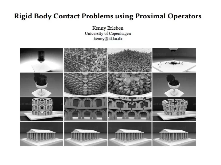
Test Scenes
Gauss-Seidel or Jacobi Variant?
Convergence rate behaviors of 424 runs of Jacks (Jacobi) 10 6 Max 3rd Quartile 10 4 Median 1st Quartile Merit function 10 2 Min 10 0 10 -2 10 -4 0 20 40 60 80 100 120 140 160 180 200 Solver iteration
Convergence rate behaviors of 424 runs of Jacks (Gauss Seidel) 10 6 Max 3rd Quartile 10 4 Median 1st Quartile Merit function 10 2 Min 10 0 10 -2 10 -4 0 20 40 60 80 100 120 140 160 180 200 Solver iteration
Divergence Count Comparison 140 Jacks (Jacobi) Spheres (Jacobi) Tower (Jacobi) 120 Wall (Jacobi) Jacks (Gauss Seidel) 100 Spheres (Gauss Seidel) Count (#) Tower (Gauss Seidel) 80 Wall (Gauss Seidel) 60 40 20 50 100 150 200 250 300 350 400 Solver run(#)
Exit Status
Blocked r-Factor 1400 Absolute Convergence 1200 Relative Convergence Observations (#) Non Convergence 1000 Divergence 800 600 400 200 0 Glasses Jacks Spheres Tower Wall Test Scenes
Global r-Factor 1400 Absolute Convergence 1200 Relative Convergence Observations (#) Non Convergence 1000 Divergence 800 600 400 200 0 Glasses Jacks Spheres Tower Wall Test Scenes
Local r-Factor 1400 Absolute Convergence 1200 Relative Convergence Observations (#) Non Convergence 1000 Divergence 800 600 400 200 0 Glasses Jacks Spheres Tower Wall Test Scenes
Iterations
Convergence rate behaviors of 424 runs of Jacks (Blocked) 10 6 Max 3rd Quartile 10 4 Median Merit function 1st Quartile 10 2 Min 10 0 10 -2 10 -4 0 50 100 150 200 250 300 350 400 450 Solver iteration
Convergence rate behaviors of 424 runs of Jacks (Global) 10 6 Max 3rd Quartile 10 4 Median Merit function 1st Quartile 10 2 Min 10 0 10 -2 10 -4 0 50 100 150 200 250 Solver iteration
Convergence rate behaviors of 424 runs of Jacks (Local) 10 6 Max 3rd Quartile 10 4 Median Merit function 1st Quartile 10 2 Min 10 0 10 -2 10 -4 0 20 40 60 80 100 120 140 160 180 200 Solver iteration
Overall Performance
Timing details of Spheres (Blocked) test scene 10 7 Solver 10 6 Collision Detection Narrow Phase 10 5 Preprocessing Time (ms) 10 4 Contact Reduction Broad Phase 10 3 10 2 10 1 10 0 0 50 100 150 200 250 300 350 400 450 Simulaiton Step (#)
Timing details of Spheres (Global) test scene 10 7 Solver 10 6 Collision Detection Narrow Phase 10 5 Preprocessing Time (ms) 10 4 Contact Reduction Broad Phase 10 3 10 2 10 1 10 0 0 50 100 150 200 250 300 350 400 450 Simulaiton Step (#)
Timing details of Spheres (Local) test scene 10 7 Collision Detection 10 6 Narrow Phase Solver 10 5 Preprocessing Time (ms) 10 4 Contact Reduction Broad Phase 10 3 10 2 10 1 10 0 0 50 100 150 200 250 300 350 400 450 Simulaiton Step (#)
Summary of Findings • Proximal operators are a flexible modeling tool for contact dynamics • Gauss-Seidel or Jacobi? • Gauss-Seidel variant is more predictable than Jacobi variant • Jacobi variant causes divergence more often than Gauss-Seidel variant • The r-Factor strategies • They only change the numerics not the model • Adaptive r-values improves convergence over constant r-values • Blocked is hopeless for our test cases • Global has advantages for structured stacks, local is slightly faster but not much
Thanks
Recommend
More recommend
Explore More Topics
Stay informed with curated content and fresh updates.
