Projective Splitting Methods for Decomposing Convex Optimization - PowerPoint PPT Presentation

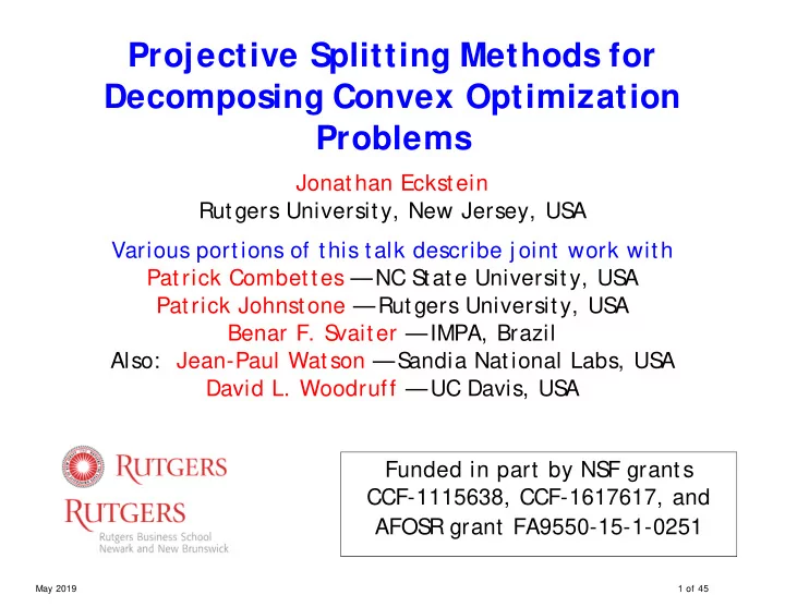
Projective Splitting Methods for Decomposing Convex Optimization Problems Jonat han Eckstein Rutgers University, New Jersey, US A Various portions of this talk describe j oint work with Patrick Combettes — NC S tate University, US A Patrick Johnstone — Rutgers University, US A Benar F. S vaiter — IMPA, Brazil Also: Jean-Paul Watson — S andia National Labs, US A David L. Woodruff — UC Davis, US A Funded in part by NSF grants CCF-1115638, CCF-1617617, and AFOS R grant FA9550-15-1-0251 May 2019 1 of 45

Introductory Remarks • I did some of the earlier work on an optimization algorithm called the ADMM (the Alternating Direction Method of Multipliers) o But not the earliest work May 2019 2 of 45

Introductory Remarks • I did some of the earlier work on an optimization algorithm called the ADMM (the Alternating Direction Method of Multipliers) o But not the earliest work • I know that the ADMM has been used in image processing because about 15 years ago I st arted being asked to referee a deluge of papers with this picture: May 2019 3 of 45

Introductory Remarks • I did some of the earlier work on an optimization algorithm called the ADMM (the Alternating Direction Method of Multipliers) o But not the earliest work • I know that the ADMM has been used in image processing because about 15 years ago I st arted being asked to referee a deluge of papers with this picture: May 2019 4 of 45

Introductory Remarks • I did some of the earlier work on an optimization algorithm called the ADMM (the Alternating Direction Method of Multipliers) o But not the earliest work • I know that the ADMM has been used in image processing because about 15 years ago I st arted being asked to referee a deluge of papers with this picture: • Today I want to talk about an algorithm t hat uses similar building blocks to the ADMM but is much more flexible May 2019 5 of 45

More General Problem Setting The algorit hms in t his talk can work for monotone inclusion problems of the form n ∈ ∑ * 0 ( ) G T G x i i i = i 1 where •    0 , , are real Hilbert spaces n •   are (generally set-valued) maximal monot one T : i i i =  operators, 1, , i n • =   are bounded linear maps,  : G i 1, , n i 0 i However, for this t alk we will restrict ourselves to... May 2019 6 of 45

A General Convex Optimization Problem { } ∑ n min ( ) f G x = i i 1 i x • For = → ∪ +∞    p , is closed proper convex i 1, , n f : { } i i • For = ×  i 1, , n , G is a p m real matrix i i • Assume you have a class of such problems t hat is not suitable for standard LP/ NLP solvers because either o The problems are very large o They is fairly large but also dense May 2019 7 of 45

Subgradient Maps of Convex Functions, Monotonicity { } ∂ of a convex function → ∪ +∞ p   The subgradient map f : is f given by { } ∂ = ≥ + − ∀ ∈  p f x ( ) y f x ( ') f x ( ) y x , ' x x ' . This has the property that ∈∂ ∈∂ ⇒ − − ≥ y f x ( ), ' y f x ( ') x x y ', y ' 0 Proof: − ≥ − f x ( ') f x ( ) y x , ' x − ≥ − f x ( ) f x ( ') y x ', x ' ≥ − − 0 y ' y x , x ' May 2019 8 of 45

Normal Cone Maps The indicat or f unct ion of a nonempty closed convex set C is ∈  0, x C δ = +∞ ( ) x ∉ C  , x C Its subgradient map is the normal cone map N of C : C { }  − ≤ ∀ ∈ ∈ y y x , ' x 0 x ' C , x C ∂ δ = = ∅ ( ) x N ( ) x C C ∉  x C y x − ≤ y x , ' x 0 C + − ≤ − ', ' 0 y x x x ' x − − ≤ y ' y x , x ' 0 x ' y ' N ( ') x C May 2019 9 of 45

A Subgradient Chain Rule • S → ∪ +∞   p uppose f : { } is closed proper convex • S × uppose G is a p real matrix m Then for any x , ) { } ( ∂ ⊇ ∂ = ∈∂  T T ( f G x )( ) G f Gx G y y f Gx ( ) and “ usually” ( ) ∂ = ∂  T ( )( ) f G x G f Gx May 2019 10 of 45

An Optimality Condition Let’ s go back to { } ∑ n min f G x ( ) = i i i 1 x ∈ ∈ ∈     p p m S uppose we have z , w , , w such that 1 n 1 n ∈∂ =  w f G z ( ) i 1, , n i i i n ∑ = T G w 0 i i = i 1 ∑   ∈∂  n  The chain rule then implies that 0 f G ( ) z , so…  = i i i 1 z is a solution t o our problem • This is always a sufficient optimality condit ion • It’ s “ usually” necessary as well • The w are the Lagrange multipliers / dual variables i May 2019 11 of 45

The Primal-Dual Solution Set (Kuhn-Tucker Set) { } ∑ n = ∀ = ∈∂ =    T ( , z w , , w ) ( i 1, n w ) f G z ( ), G w 0 1 = n i i i i i i 1 = = Or, if we assume that p m G , Id  , n n m { } ∑ − 1 = ∀ = − ∈∂ − n ∈∂    T ( , z w , , w ) ( i 1, n 1) w f G z ( ), G w f ( ) z − = 1 n 1 i i i i i n i 1 • This is t he set of points satisfying the optimality conditions • S tanding assumption:  is nonempt y • Essentially in E & S vaiter 2009:  is a closed convex set • In the = = p m G , Id  case, streamline notation: m n n − ∑ − n 1 ∈ × ×     * For , let w G w w n − = 1 1 n i i i 1 May 2019 12 of 45

Valid Inequalities for  • Take some x y ∈  such t hat ∈∂ =  p for , y f x ( ) i 1, , n i i i i i i • If ( , ∈  ∈∂ =  z ) , then w f G z ( ) for i 1, , n w i i i • S − − ≥ =  o, for 1, , x G z y , w 0 i n i i i i • Negate and add up: n ∑ ϕ = − − ≤ ∀ ∈  ( , z ) G z x , y w 0 ( , z ) w w i i i i = i 1 { } = ϕ = H p ( ) p 0  ϕ ≤ ∀ ∈  ( ) p 0 p May 2019 13 of 45

Confirming that ϕ is Affine ϕ The quadratic terms in ( , w take the form z ) n n n ∑ ∑ ∑ − = − = − = − = T T G z , w z , G w z , G w z , 0 0 i i i i i i = = = i 1 i 1 i 1 • Also true in the = = th , Id  case where we drop the n p m G m n n index o S lightly different proof, same basic idea May 2019 14 of 45

Generic Projection Method for a Closed Convex Set  in a Hilbert Space  Apply the following general template: • Given p ∈  , choose some affine function ϕ with k k ϕ ≤ ∀ ∈  k p ( ) 0 p { } • Proj ect = ϕ = k p onto , possibly with an H p ( ) p 0 k k λ ∈ ε − ε overrelaxation factor [ ,2 ] , giving p + , and repeat… k k 1 p k ϕ p + is affine k 1 k { } = ϕ = H p ( ) p 0 k k ϕ ≤ ∀ ∈  ( ) p 0 p  k ϕ > ( p ) 0 k k ϕ by picking some = × × ×      p p m In our case: and we find n 1 k ∈ ∈∂ =   k k p k k x , y : y f x ( ), i 1, , n and using the construction above i i i i i i May 2019 15 of 45

General Properties of Projection Algorithms ≠ ∅  Proposition. In such algorithms, assuming t hat , • { } − p ∈  k * * p p is nonincreasing for all • { k p } is bounded + − • → k 1 k p p 0 { } • If { ∇ ϕ ϕ ≤ k is bounded, then } limsup ( p ) 0 k k →∞ k • If all limit points of { k are in  , then { k p } p } converges to a point in  ϕ The first t hree properties hold no matter how badly we choose k ϕ so that the st ipulations of the last two The idea is to pick k properties hold – t hen we have a convergent algorit hm ϕ badly, we may “ stall” If we pick k May 2019 16 of 45

ϕ Selecting the Right k • S ϕ involves picking some ∈ ∈∂  p k k k k electing x , y : y f x ( ) , i k i i i i i =  i 1, , n • It turns out there are many ways to pick k k x , y so that the last i i two properties of t he proposition are satisfied • One fundamental t hing we would like is n ∑ ϕ − − ≥  k k k k k k ( , ) , 0 z G z x y w w k i i i i = i 1 ∉  k k with strict inequality if ( z , ) w • The oldest suggestion is “ prox” (E & S vait er 2008 & 2009) May 2019 17 of 45

The Prox Operation { } • S → ∪ +∞ p   uppose we have a convex function : f • Take any vector r ∈  and scalar c > and solve p 0   1 = + − 2   argmin ( ') ' x f x x r   2 c ∈ p  x ' • Optimality condition for this minimization is 1 ∈∂ + − 0 ( ) ( ) f x x r c 1 ( • S − ∈∂  o we have y r x ) f x ( ) c 1 ( • And + = + ⋅ − = x cy x c r x ) r c • S x y ∈  such that ∈∂ + = p o, we j ust found , and x cy r y f x ( ) • Call this Prox ( ) c f r ∂ May 2019 18 of 45