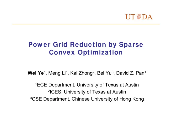
UT DA Pow er Grid Reduction by Sparse Convex Optimization Wei Ye 1 - PowerPoint PPT Presentation
UT DA Pow er Grid Reduction by Sparse Convex Optimization Wei Ye 1 , Meng Li 1 , Kai Zhong 2 , Bei Yu 3 , David Z. Pan 1 1 ECE Department, University of Texas at Austin 2 ICES, University of Texas at Austin 3 CSE Department, Chinese University of
UT DA Pow er Grid Reduction by Sparse Convex Optimization Wei Ye 1 , Meng Li 1 , Kai Zhong 2 , Bei Yu 3 , David Z. Pan 1 1 ECE Department, University of Texas at Austin 2 ICES, University of Texas at Austin 3 CSE Department, Chinese University of Hong Kong
On-chip Pow er Delivery Netw ork Power grid › Multi-layer mesh structure › Supply power for on-chip devices Power grid verification › Verify current density in metal wires (EM) › Verify voltage drop on the grids › More expensive due to increasing sizes of grids » e.g., 10M nodes, >3 days [Yassine+, ICCAD’16] 1
Modeling Pow er Grid Circuit modeling › Resistors to represent metal wires/vias › Current sources to represent current drawn by underlying devices › Voltage sources to represent external power supply › Transient: capacitors are attached from each node to ground Port node: node attached current/voltage sources Non-port node: only has internal connection Voltage source Current source Port node Non-port node 2
Linear System of Pow er Grid Resistive grid model: �� � � › � is � � � Laplacian matrix (symmetric and diagonally- dominant): › � �,� denotes a physical conductance between two nodes � and � A power grid is safe, if ∀� : � � � � �� Long runtime to solve �� � � for large linear systems 3
Previous Work Power grid reduction › Reduce the size of power grid while preserving input- output behavior › Trade-off between accuracy and reduction size Topological methods › TICER [Sheehan+, ICCAD’99] › Multigrid [Su+, DAC’03] › Effective resistance [Yassine+, ICCAD’16] Numerical methods › PRIMA [Odabasioglu+, ICCAD’97] › Random sampling [Zhao+, ICCAD’14] › Convex optimization [Wang+, DAC’15] 4
Problem Definition Input: › Large power grid › Current source values Output: reduced power grid › Small › Sparse (as input grid) › Keep all the port nodes › Preserve the accuracy in terms of voltage drop error 5
Overall Flow Node and edge set generation Large graph partition For each subgraph: Node elimination by Schur complement Edge sparsification by GCD Store reduced nodes and edges 6
Node Elimination Linear system: �� � � � can be represented as a 2 � 2 block-matrix: � � � �� � �� � � �� � �� � and � can be represented as follows: � � � � � � and � � � � 0 Applying Schur complement on the DC system: � � � �� � � �� � �� �� � �� � � which satisfies: �� � � � � � 7
Node Elimination (cont’d) Node Elimination Edge Sparsification Output graph keeps all the nodes of interest Output graph is dense Edge sparsification: sparsify the reduced Laplacian without losing accuracy 8
Edge Sparsification Goal of edge sparsification › Accuracy › Sparsity reduce the nonzero elements off-the-diagonal in L Formulation (1): Formulation (2): [Wang+, DAC2014] L2 norm L1 norm 9
Edge Sparsification Formulation (2): [DAC2014 Wang+] Problem : accuracy on the Vdd node does not guarantee accuracy on the current source nodes Formulation (3): › Weight vector: › Strongly convex and coordinate-wise Lipschitz smooth 10
Coordinate Descent (CD) Method Update one coordinate at each iteration Coordinate descent: Set � � 1 and � � � 0 For a fixed number of iterations (or convergence is reached): Choose a coordinate ��, �� Compute the step size � ∗ by minimizing argmin f�� � �� �,� � � � � � ∗ ��� ← � �,� Update � �,� How to decide the coordinate? › Cyclic (CCD) › Random sampling (RCD) › Greedy coordinate descent (GCD) 11
CD vs Gradient Descent Gradient descent (GD) algorithm: � ��� ← � � � ������ GD/SGD update ��� � � elements in � and gradient matrix � at each iteration CD updates � 1 elements in � (Laplacian property) CD proves to update � � elements in � for Formulation (2) and (3). 12
Greedy Coordinate Descent (GCD) Input L Max-heap Output X 13
GCD vs CCD Input graph GCD: CCD: Add an edge Update an edge Iteration T Iteration 1 Iteration 2 Iteration 3 Iteration 4 GCD produces sparser results › CCD (RCD) goes through all coordinates repeatedly › GCD selects the most significant coordinates to update 10 5 CCD GCD 10 4 Edge Count 10 3 10 2 10 1 10 0 0 5 10 15 20 Edge Weight 14
GCD Coordinate Selection General Gauss-Southwell Rule: Observation: the objective function is quadratic w.r.t. the chosen coordinate GCD is stuck for some corner cases: A new coordinate selection rule: 15
GCD Speedup Time complexity is ��� � � per iteration › traverse ��� � � elements to get the best index › As expensive as gradient descent Observation: each node has at most � neighbors → heap Heap to store ��� � � elements in � : › Pick the largest gradient, ��1� › Update ���� elements, ��� log �� Lookup table › ��� � � space; � 1 for each update Improved time complexity ��� log �� 16
Experimental Results Sparsity and accuracy trade-off Accuracy and runtime trade-off 17
Gradient Descent Comparison Sparsity Accuracy Runtime 18
Experimental Results CKT ibmpg2 ibmpg3 ibmpg4 ibmpg5 ibmpg6 #Port Before 19,173 100,988 133,622 270,577 380,991 Nodes After 19,173 100,988 133,622 270,577 380,991 #Non-port Before 46,265 340,088 345,122 311,072 481,675 Nodes After 0 0 0 0 0 #Edges Before 106,607 724,184 779,946 871,182 1283,371 After 48,367 243,011 284,187 717,026 935,322 Error 1.2% 0.7% 4.8% 2.2% 2.0% Runtime 38s 106s 132s 123s 281s 19
Conclusion Main Contributions: › An iterative power grid reduction framework › Weighted convex optimization-based formulation › A GCD algorithm with optimality guarantee and runtime efficiency for edge sparsification Future Work: › Extension to RC grid reduction 20
Thanks
Recommend
More recommend
Explore More Topics
Stay informed with curated content and fresh updates.
