
Using follow-up data to adjust for selective non-participation in - PowerPoint PPT Presentation
Research problem Data Bayesian modelling Summary Using follow-up data to adjust for selective non-participation in cross-sectional setting Juho Kopra University of Jyv askyl a Department of Mathematics and Statistics NoPaHES-project
Research problem Data Bayesian modelling Summary Using follow-up data to adjust for selective non-participation in cross-sectional setting Juho Kopra University of Jyv¨ askyl¨ a Department of Mathematics and Statistics NoPaHES-project 30th August 2017 1 Juho Kopra 30th August 2017
Research problem Data Bayesian modelling Summary Research problem Data from cross-sectional surveys (Finrisk studies) No re-contact data is available for 1972-2002. → Previous solution cannot be used. Instead, we utilize the follow-up data about the smoking-related diseases: Lung cancer and Chronic Obstructive Pulmonary Disease (COPD, keuhkoahtaumatauti in Finnish). 2 Juho Kopra 30th August 2017
Research problem Data Bayesian modelling Summary Data we utilized from FINRISK studies: People aged 25-59 years-old (30-59 years-old for 1972 and 1977). Data from 1972, 1977, 1982, 1987, 1992, 1997, 2002 and 2007. We use two areas of Finland: Northern Karelia and North Savonia. In total, the data contain 52,325 persons including 9,928 persons with missing smoking indicator. 3 Juho Kopra 30th August 2017
Research problem Data Bayesian modelling Summary Variables provided by FINRISK survey samples Background knowledge for both participants and non-participants: Area, Age, Gender and Study year. Self-reported indicator of daily smoking. 4 Juho Kopra 30th August 2017
Research problem Data Bayesian modelling Summary Combining information from the National Hospitalization Register and Cause of Death Register, we build a follow-up: Up to the end of 2012. Available for both participants and non-participants. Persons age at the time of diagnosis (lung cancer or COPD). Death to other causes and the end of the follow-up are treated as censoring. → Persons with no diagnosis have censoring. 5 Juho Kopra 30th August 2017
Research problem Data Bayesian methodology (very) briefly Bayesian modelling Modelling using survival data and Bayesian modelling Summary Bayesian modelling 6 Juho Kopra 30th August 2017
Research problem Data Bayesian methodology (very) briefly Bayesian modelling Modelling using survival data and Bayesian modelling Summary Bayesian methodology (very) briefly Bayesian approach combines the information provided by the data (via likelihood function) and subjective information about parameters of the model (via prior distribution). The scientist decides the prior distributions he wants to use. Results are called posterior distribution, which represents the combination of prior and the data. 7 Juho Kopra 30th August 2017
Research problem Data Bayesian methodology (very) briefly Bayesian modelling Modelling using survival data and Bayesian modelling Summary We utilized uninformative priors for most of the parameters (not all). The informative priors we used allow identifiability of our model while restricting the unrealistic posterior prevalences. 8 Juho Kopra 30th August 2017
Modelling 1/2 Use Bayesian modelling to estimate smoking prevalence based on the survival (follow-up) data. Build a model from three submodels: 1. Participation M given smoking Y and background information X : P ( M | X, Y ) 2. Smoking Y given the background information X : P ( Y | X ) . 3. Survival model for lung cancer or COPD disease age T given smoking Y and background information X : P ( T | X, Y ) Define an informative prior regarding submodel 1 to allow identifiability, and estimate the posterior for smoking prevalence. Fit the model and simultaneously impute the missing smoking indicators ˜ Y ∼ P ( Y | M = 0 , X, T ) 9
Research problem Data Bayesian methodology (very) briefly Bayesian modelling Modelling using survival data and Bayesian modelling Summary Modelling 2/2 Participation P ( M | X, Y ) is modelled using a logistic distribution explained by gender, study year, age, region and smoking Smoking P ( Y | X ) is modelled using a logistic distribution explained by year of birth. Coefficients vary by gender, region and study year. Survival model for follow-up data P ( T | X, Y ) uses piecewise constant hasard model. The survival is explained by gender and smoking. 10 Juho Kopra 30th August 2017
Research problem Data Bayesian methodology (very) briefly Bayesian modelling Modelling using survival data and Bayesian modelling Summary Prior distributions Participation model: Informative prior is required for the ” η ” which models how smoking affects participation. η ∼ Logistic ( µ = 0 , s = 2 . 05 − 1 ) Risk factor model: Uninformative priors; N (0 , 1000) . Survival model: Baseline hasard is a priori monotonically increasing. Others are uninformative priors; N (0 , 1000) . 11 Juho Kopra 30th August 2017
Research problem Data Bayesian methodology (very) briefly Bayesian modelling Modelling using survival data and Bayesian modelling Summary Model fitting Models were implemented with Just Another Gibbs Sampler -software (JAGS). (Plummer, 2003) The imputations for smoking indicator Y i are drawn from fully conditional distribution P ( Y i | M i = 0 , X i , T i ) . The model fitting took 107 hours to complete (five days). The high absolute number of missing values (9,928) and computationally intensive algorithm (MCMC) explains the long running time. 12 Juho Kopra 30th August 2017
Research problem Data Bayesian methodology (very) briefly Bayesian modelling Modelling using survival data and Bayesian modelling Summary Simulation experiment We generated randomly one data from the model we use. Model appears to be able to restore the original trends from the data. 13 Juho Kopra 30th August 2017
Trend estimates for the simulated data: North Karelia men North Karelia women 0.55 0.40 participants only ● true trends 0.50 0.35 ● Bayesian modelling 95 % credible interval 0.45 0.30 proportion of smokers proportion of smokers ● 0.40 0.25 0.35 ● 0.20 ● ● ● ● ● ● ● 0.30 0.15 ● ● ● ● ● 0.25 0.10 ● 0.20 0.05 1972 1982 1992 2002 1972 1982 1992 2002 Northern Savonia men Northern Savonia women 0.55 0.40 0.50 0.35 ● ● 0.45 0.30 proportion of smokers ● proportion of smokers ● 0.40 0.25 ● ● ● 0.35 0.20 ● ● ● 0.30 0.15 ● ● ● ● ● 0.25 0.10 ● 0.20 0.05 1972 1982 1992 2002 1972 1982 1992 2002 14
Trend estimates for the FINRISK data: North Karelia men North Karelia women 0.55 0.30 participants only ● ● Bayesian modelling 0.50 95 % credible interval 0.25 0.45 proportion of smokers proportion of smokers ● ● 0.20 0.40 ● 0.35 ● ● 0.15 ● ● ● ● ● 0.30 ● ● ● ● 0.10 0.25 ● 0.20 0.05 1972 1982 1992 2002 1972 1982 1992 2002 Northern Savonia men Northern Savonia women 0.55 0.30 0.50 ● 0.25 0.45 proportion of smokers proportion of smokers ● ● 0.20 0.40 ● ● ● ● ● 0.35 ● ● 0.15 ● ● 0.30 ● ● ● 0.10 ● 0.25 0.20 0.05 1972 1982 1992 2002 1972 1982 1992 2002 15
Research problem Data Bayesian modelling Summary Summary Follow-up data can be used in Bayesian modelling to estimate the prevalence of smoking although the survey data suffer from selective non-participation. Long register-based follow-up is required. For the later years, which do not have lengthy follow-up, modelling assumptions can be made to provide different scenarios. (2007 and 2012 luckily have re-contact data) Bayesian model fitting requires informative prior and is computationally very demanding with large absolute amount of missing values. 16 Juho Kopra 30th August 2017
Research problem Data Bayesian modelling Summary THANKS 17 Juho Kopra 30th August 2017
Research problem Data Bayesian modelling Summary References Bayesian models for data missing not at random in health examination surveys . Juho Kopra, Juha Karvanen and Tommi H¨ ark¨ anen. Accepted for publication in Statistical Modelling . https://arxiv.org/abs/1610.03687 Plummer, M. (2003). JAGS: A program for analysis of Bayesian graphical models using Gibbs sampling. In Proceedings of the 3rd international workshop on distributed statistical computing. 124, p. 125. Wien, Austria: Technische Universit at Wien. 18 Juho Kopra 30th August 2017
Recommend


More recommend
Explore More Topics
Stay informed with curated content and fresh updates.