SLIDE 1 CS140 V-1
✬ ✫ ✩ ✪
Use of parallel matrix algorithms for Laplace partial differential equations
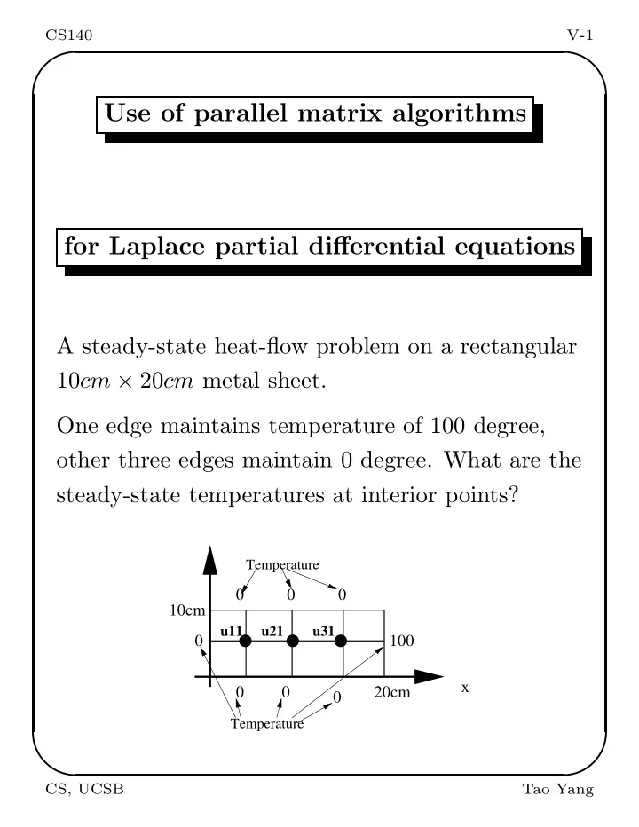
A steady-state heat-flow problem on a rectangular 10cm × 20cm metal sheet. One edge maintains temperature of 100 degree,
- ther three edges maintain 0 degree. What are the
steady-state temperatures at interior points?
100
Temperature
x
Temperature
10cm 20cm
u11 u21 u31
CS, UCSB Tao Yang
SLIDE 2 CS140 V-2
✬ ✫ ✩ ✪
The mathematical model
Laplace equation: ∂2U(x, y) ∂x2 + ∂2u(x, y) ∂y2 = 0 with the boundary condition: u(x, 0) = 0, u(x, 10) = 0. u(0, y) = 0, u(20, y) = 100. Finite difference method to solve this PDE:
- Discretize the region: Divide the function
domain into a grid with gap h at each axis.
- At each point (ih, jh), let u(ih, jh) = ui,j.
Setup a linear equation using an approximated formula for numerical differentiation.
- Solve the linear equations to find values of all
points ui,j.
CS, UCSB Tao Yang
SLIDE 3 CS140 V-3
✬ ✫ ✩ ✪
Approximating numerical differentiation
f′(x) ≈ f(x + h) − f(x) h
- r f′(x) ≈ f(x) − f(x − h)
h f′′(x) ≈ f′(x + h) − f′(x) h ≈
f(x+h)−f(x) h
+ f(x)−f(x−h)
h
h Thus f′′(x) ≈ f(x + h) + f(x − h) − 2f(x) h2 Then ∂2u(xi, yi) ∂x2 ≈ ui+1,j − 2ui,j + ui−1,j h2 ∂2u(xi, yi) ∂y2 ≈ ui,j+1 − 2ui,j + ui,j−1 h2 Adding the above two equations ui+1,j − 2uij + ui−1,j + ui,j+1 − 2ui,j + ui,j−1 = 0 Then 4ui,j − ui+1,j − ui−1,j − ui,j+1 − ui,j−1 = 0
CS, UCSB Tao Yang
SLIDE 4
CS140 V-4
✬ ✫ ✩ ✪
Example of Derived Linear Heat Equations
100
Temperature
x
Temperature
10cm 20cm
u11 u21 u31
For this case: Let u11 = x1, u21 = x2, u31 = x3. At u11, 4x1 − 0 − 0 − x2 = 0 At u21, 4x2 − x1 − 0 − x3 − 0 = 0 At u31, 4x3 − x2 − 0 − 100 − 0 = 0
4 −1 −1 4 −1 −1 4
x1 x2 x3
=
100
Solutions: x1 = 1.786, x2 = 7.143, x3 = 26.786
CS, UCSB Tao Yang
SLIDE 5
CS140 V-5
✬ ✫ ✩ ✪
Linear heat equations for a general 2D grid
Given a general (n + 2) × (n + 2) grid, we have n2 equations: 4ui,j − ui+1,j − ui−1,j − ui,j+1 − ui,j−1 = 0 for 1 ≤ i, j ≤ n. Or express them as: ui,j = (ui+1,j + ui−1,j + ui,j+1 + ui,j−1)/4 Example, r = 2, n = 6.
Temperature held at U Temperature held at U1 held at U Temperature held at U Temperature
CS, UCSB Tao Yang
SLIDE 6
CS140 V-6
✬ ✫ ✩ ✪
We order the unknowns as (u11, u12, · · · , u1n, u21, u22, · · · , u2n, · · · , un1, · · · , unn) For n = 2, the ordering is:
x1 x2 x3 x4
=
u11 u12 u21 u22
The matrix is:
4 −1 −1 −1 4 −1 −1 4 −1 −1 −1 4
x1 x2 x3 x4
=
u01 + u10 u20 + u31 u02 + u13 u32 + u23
CS, UCSB Tao Yang
SLIDE 7
CS140 V-7
✬ ✫ ✩ ✪
In general, the left side matrix is:
T −I −I T −I −I T −I ... ... ... −I T
n2×n2
T =
4 −1 −1 4 −1 −1 4 −1 ... ... ... −1 4
n×n
CS, UCSB Tao Yang
SLIDE 8
CS140 V-8
✬ ✫ ✩ ✪
I =
1 1 1 ... 1
n×n
The matrix is too sparse, direct methods for solving this system takes too much time.
CS, UCSB Tao Yang
SLIDE 9
CS140 V-9
✬ ✫ ✩ ✪
The Jacobi Iterative Method
Given 4ui,j − ui+1,j − ui−1,j − ui,j+1 − ui,j−1 = 0 for 1 ≤ i, j ≤ n. The Jacobi program: Repeat For i=1 to n For j=1 to n unew
i,j
= 0.25(ui+1,j + ui−1,j + ui,j+1 + ui,j−1). EndFor EndFor Until unew
ij
− uij < ǫ Called 5-point stencil computation as ui,j depends on 4 neighbors.
CS, UCSB Tao Yang
SLIDE 10
CS140 V-10
✬ ✫ ✩ ✪
The Gauss-Seidel Method
Repeat uold = u. For i=1 to n For j=1 to n ui,j = 0.25(ui+1,j + ui−1,j + ui,j+1 + ui,j−1). EndFor EndFor Until uij − uold
ij < ǫ
CS, UCSB Tao Yang
SLIDE 11
CS140 V-11
✬ ✫ ✩ ✪
Parallel Jacobi Method
Assume we have a mesh of n × n processors. Assign ui,j to processor pi,j. The SPMD Jacobi program at processor pi,j: Repeat Collect data from four neighbors: ui+1,j, ui−1,j, ui,j+1, ui,j−1 from pi+1,j, pi−1,j, pi,j+1, pi,j−1. unew
i,j
= 0.25(ui+1,j + ui−1,j + ui,j+1 + ui,j−1). diffi,j = |unew
ij
− uij| Do a global reduction to get the maximum of diffi,j as M. Until M < ǫ
CS, UCSB Tao Yang
SLIDE 12 CS140 V-12
✬ ✫ ✩ ✪
Performance evaluation
- Each computation step takes ω = 5 operations.
- There are 4 communication messages to be
- received. Assume sequential receiving.
Communication costs 4(α + β).
- Assume that the global reduction takes
(α + β) log n.
- The sequential time Seq = Kωn2 where K is the
number of steps.
ω = 0.5, β = 0.1, α = 100, n = 500, p2 = 2500.
PT = K(ω + (4 + log n)(α + β)) Speedup = ω ∗ n2 ω + (4 + log n)(α + β) ≈ 192 Efficiency = Speedup n2 = 7.7%.
CS, UCSB Tao Yang
SLIDE 13 CS140 V-13
✬ ✫ ✩ ✪
Grid partitioning
- Reduce the number of processors. Increase the
granularity of computations.
- Map the n × n grid to processors using 2D block
method. Assume a p × p mesh,γ = n
p .
Example, r = 2, n = 6.
Temperature held at U Temperature held at U1 held at U Temperature held at U Temperature
CS, UCSB Tao Yang
SLIDE 14
CS140 V-14
✬ ✫ ✩ ✪
Code partitioning
Re-write the kernel part of the sequential code as: For bi = 1 to p For bj = 1 to p For i = (bi − 1)γ + 1 to biγ For j = (bj − 1)γ + 1 to bjγ unew
i,j
= 0.25(ui+1,j + ui−1,j + ui,j+1 + ui,j−1). EndFor EndFor EndFor EndFor
CS, UCSB Tao Yang
SLIDE 15
CS140 V-15
✬ ✫ ✩ ✪
Parallel SPMD code
On processor pbi,bj: Repeat Collect the data from its four neighbors. For i = (bi − 1)γ + 1 to biγ For j = (bj − 1)γ + 1 to bjγ unew
i,j
= 0.25(ui+1,j + ui−1,j + ui,j+1 + ui,j−1). EndFor EndFor Compute the local maximum diffbi,bj for the difference between old values and new values. Do a global reduction to get the maximum diffbi,bj as M. Until M < ǫ
CS, UCSB Tao Yang
SLIDE 16 CS140 V-16
✬ ✫ ✩ ✪
Performance evaluation
- At each processor, each computation step takes
ωr2 operations.
- The communication cost is 4(α + rβ).
- Assume that the global reduction takes
(α + β) log p.
- The number of steps is K.
- Assume ω = 0.5, β = 0.1, α = 100, n = 500, r =
100, p2 = 25. PT = K(r2ω + (4 + log p)(α + rβ)) Speedup = ωr2p2 r2ω + (4 + log p)(α + rβ) ≈ 21.2. Efficiency = 84%.
CS, UCSB Tao Yang
SLIDE 17 CS140 V-17
✬ ✫ ✩ ✪
Red-Black Ordering
Reordering variables to eliminate most of data dependence in the Gauss Seidel algorithm.
- Points are divided into “red” points (white)
and black points.
- First, black points are computed (using the
- ld red point values).
- Second, red points are computed (using the
new black point values).
CS, UCSB Tao Yang
SLIDE 18 CS140 V-18
✬ ✫ ✩ ✪
Parallel code for red-black ordering
- Point (i,j) is black if i+j is even.
- Point (i,j) is red if i+j is odd.
- Computation on black points (stage 1) can be
done in parallel.
- Computation on red points (stage 2) can be
done in parallel. Parallel Code (Kernel)
- For all points (i,j) with (i+j) mod 2=0, do in
parallel ui,j = 0.25(ui+1,j+ui−1,j+ui,j+1+ui,j−1).
- For all points (i,j) with (i+j) mod 2=1, do in
parallel ui,j = 0.25(ui+1,j+ui−1,j+ui,j+1+ui,j−1).
CS, UCSB Tao Yang