Unit 4: Inference for numerical variables Lecture 3: ANOVA - - PowerPoint PPT Presentation

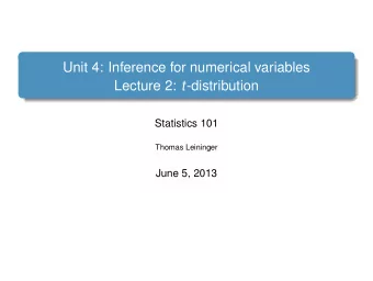
Unit 4: Inference for numerical variables Lecture 3: ANOVA

Statistics 101

Thomas Leininger

June 10, 2013

Announcements

Announcements

Proposals due tomorrow. Will be returned to you by Wednesday. You MUST complete the proposal process. A few things to watch out for:

Data is plural, data set is singular. Avoid using population data - if you have population data, you might consider taking a random sample. Exploratory analysis: should include some summary statistics and some graphics AND interpretations. If using existing data, find out how your data were collected, and discuss the sampling method as well as any possible biases. Scope of inference: generalizability & causality.

Statistics 101 (Thomas Leininger) U4 - L3: ANOVA June 10, 2013 2 / 34

ANOVA Aldrin in the Wolf River

The Wolf River in Tennessee flows past an abandoned site once used by the pesticide industry for dumping wastes, including chlordane (pesticide), aldrin, and dieldrin (both insecticides). These highly toxic organic compounds can cause various cancers and birth defects. The standard methods to test whether these substances are present in a river is to take samples at six-tenths depth. But since these compounds are denser than water and their molecules tend to stick to particles of sediment, they are more likely to be found in higher concentrations near the bottom than near mid-depth.

Statistics 101 (Thomas Leininger) U4 - L3: ANOVA June 10, 2013 3 / 34

ANOVA Aldrin in the Wolf River

Data

Aldrin concentration (nanograms per liter) at three levels of depth. aldrin depth 1 3.80 bottom 2 4.80 bottom ... 10 8.80 bottom 11 3.20 middepth 12 3.80 middepth ... 20 6.60 middepth 21 3.10 surface 22 3.60 surface ... 30 5.20 surface

Statistics 101 (Thomas Leininger) U4 - L3: ANOVA June 10, 2013 4 / 34

ANOVA Aldrin in the Wolf River

Exploratory analysis

Aldrin concentration (nanograms per liter) at three levels of depth.

bottom middepth surface 3 4 5 6 7 8 9

n mean sd bottom 10 6.04 1.58 middepth 10 5.05 1.10 surface 10 4.20 0.66

• verall

30 5.1 0 1.37

Statistics 101 (Thomas Leininger) U4 - L3: ANOVA June 10, 2013 5 / 34

ANOVA Aldrin in the Wolf River

Research question

Is there a difference between the mean aldrin concentrations among the three levels? To compare means of 2 groups we use a Z or a T statistic. To compare means of 3+ groups we use a new test called ANOVA and a new statistic called F.

Statistics 101 (Thomas Leininger) U4 - L3: ANOVA June 10, 2013 6 / 34

ANOVA Aldrin in the Wolf River

Recap: 2-sample CIs and HTs

n mean sd bottom 10 6.04 1.58 middepth 10 5.05 1.10 surface 10 4.20 0.66

• verall

30 5.1 0 1.37 HT: Tdf = (¯

x1−¯ x2)−null value SE

where SE =

• s2

1

n1 + s2

2

n2 and

df = min(n1 − 1, n2 − 1) CI: (¯ x1 − ¯ x2) ± t⋆

df × SE

Application exercise: Perform a HT and construct a CI for each difference.

Statistics 101 (Thomas Leininger) U4 - L3: ANOVA June 10, 2013 7 / 34

ANOVA Aldrin in the Wolf River

ANOVA

ANOVA is used to assess whether the mean of the outcome variable is different for different levels of a categorical variable. H0 : The mean outcome is the same across all categories,

µ1 = µ2 = · · · = µk,

where µi represents the mean of the outcome for observations in category i. HA : At least one mean is different than others.

Statistics 101 (Thomas Leininger) U4 - L3: ANOVA June 10, 2013 8 / 34

ANOVA Aldrin in the Wolf River

Conditions

1

The observations should be independent within and between groups

If the data are a simple random sample, this condition is satisfied. Carefully consider whether the between-group data is independent (e.g. no pairing). Always important, but sometimes difficult to check.

2

The observations within each group should be nearly normal.

Especially important when the sample sizes are small.

How do we check for normality?

3

The variability across the groups should be about equal.

Especially important when the sample sizes differ between groups.

How can we check this condition?

Statistics 101 (Thomas Leininger) U4 - L3: ANOVA June 10, 2013 9 / 34

ANOVA Aldrin in the Wolf River

z/t test vs. ANOVA - Purpose

z/t test Compare means from two groups to see whether they are so far apart that the observed difference cannot reasonably be attributed to sampling variability. H0 : µ1 = µ2 HA : µ1 µ2 HA : µ1 < µ2 HA : µ1 > µ2 ANOVA Compare the means from two or more groups to see whether they are so far apart that the observed differences cannot all reasonably be attributed to sampling variability. H0 : µ1 = µ2 = · · · = µk HA : At least one mean is different

Statistics 101 (Thomas Leininger) U4 - L3: ANOVA June 10, 2013 10 / 34

ANOVA Aldrin in the Wolf River

z/t test vs. ANOVA - Method

z/t test Compute a test statistic (a ratio). z/t = (¯ x1 − ¯ x2) − (µ1 − µ2) SE(¯ x1 − ¯ x2) ANOVA Compute a test statistic (a ratio). F = variability bet. groups variability w/in groups Large test statistics lead to small p-values. If the p-value is small enough H0 is rejected, and we conclude that the population means are not equal.

Statistics 101 (Thomas Leininger) U4 - L3: ANOVA June 10, 2013 11 / 34

ANOVA Aldrin in the Wolf River

z/t test vs. ANOVA

With only two groups t-test and ANOVA are equivalent, but only if we use a pooled standard variance in the denominator of the test statistic. With more than two groups, ANOVA compares the sample means to an overall grand mean.

Statistics 101 (Thomas Leininger) U4 - L3: ANOVA June 10, 2013 12 / 34

ANOVA Aldrin in the Wolf River

Hypotheses

Question What are the correct hypotheses for testing for a difference between the mean aldrin concentrations among the three levels? (a) H0 : µB = µM = µS HA : µB µM µS (b) H0 : µB µM µS HA : µB = µM = µS (c) H0 : µB = µM = µS HA : At least one mean is different. (d) H0 : µB = µM = µS = 0 HA : At least one mean is different. (e) H0 : µB = µM = µS HA : µB > µM > µS

Statistics 101 (Thomas Leininger) U4 - L3: ANOVA June 10, 2013 13 / 34

ANOVA ANOVA and the F test

Test statistic

Does there appear to be a lot of variability within groups? How about between groups? F = variability bet. groups variability w/in groups

Statistics 101 (Thomas Leininger) U4 - L3: ANOVA June 10, 2013 14 / 34

ANOVA ANOVA and the F test

F distribution and p-value

F = variability bet. groups variability w/in groups In order to be able to reject H0, we need a small p-value, which requires a large F statistic. In order to obtain a large F statistic, variability between sample means needs to be greater than variability within sample means.

Statistics 101 (Thomas Leininger) U4 - L3: ANOVA June 10, 2013 15 / 34

ANOVA ANOVA output, deconstructed

Df Sum Sq Mean Sq F value Pr(>F) (Group) depth 2 16.96 8.48 6.13 0.0063 (Error) Residuals 27 37.33 1.38 Total 29 54.29

Degrees of freedom associated with ANOVA groups: dfG = k − 1, where k is the number of groups total: dfT = n − 1, where n is the total sample size error: dfE = dfT − dfG dfG = k − 1 = 3 − 1 = 2 dfT = n − 1 = 30 − 1 = 29 dfE = 29 − 2 = 27

Statistics 101 (Thomas Leininger) U4 - L3: ANOVA June 10, 2013 16 / 34

ANOVA ANOVA output, deconstructed

Df Sum Sq Mean Sq F value Pr(>F) (Group) depth 2 16.96 8.48 6.13 0.0063 (Error) Residuals 27 37.33 1.38 Total 29 54.29

Sum of squares between groups, SSG Measures the variability between groups SSG =

k

• i=1

ni(¯ xi − ¯ x)2 where ni is each group size, ¯ xi is the average for each group, ¯ x is the

• verall (grand) mean.

n mean bottom 10 6.04 middepth 10 5.05 surface 10 4.2

• verall

30 5.1

SSG

=

• 10 × (6.04 − 5.1)2

+

• 10 × (5.05 − 5.1)2

+

• 10 × (4.2 − 5.1)2

=

16.96

Statistics 101 (Thomas Leininger) U4 - L3: ANOVA June 10, 2013 17 / 34

ANOVA ANOVA output, deconstructed

Df Sum Sq Mean Sq F value Pr(>F) (Group) depth 2 16.96 8.48 6.13 0.0063 (Error) Residuals 27 37.33 1.38 Total 29 54.29

Sum of squares total, SST Measures the total variability SST =

n

• i=1

(xi − ¯

x) where xi represents each observation in the dataset. SST

= (3.8 − 5.1)2 + (4.8 − 5.1)2 + (4.9 − 5.1)2 + · · · + (5.2 − 5.1)2 = (−1.3)2 + (−0.3)2 + (−0.2)2 + · · · + (0.1)2 =

1.69 + 0.09 + 0.04 + · · · + 0.01

=

54.29

Statistics 101 (Thomas Leininger) U4 - L3: ANOVA June 10, 2013 18 / 34

ANOVA ANOVA output, deconstructed

Df Sum Sq Mean Sq F value Pr(>F) (Group) depth 2 16.96 8.48 6.13 0.0063 (Error) Residuals 27 37.33 1.38 Total 29 54.29

Sum of squares error, SSE Measures the variability within groups: SSE = SST − SSG SSE = 54.29 − 16.96 = 37.33

Statistics 101 (Thomas Leininger) U4 - L3: ANOVA June 10, 2013 19 / 34

ANOVA ANOVA output, deconstructed

Df Sum Sq Mean Sq F value Pr(>F) (Group) depth 2 16.96 8.48 6.13 0.0063 (Error) Residuals 27 37.33 1.38 Total 29 54.29

Mean square error Mean square error is calculated as sum of squares divided by the de- grees of freedom. MSG

=

16.96/2 = 8.48 MSE

=

37.33/27 = 1.38

Statistics 101 (Thomas Leininger) U4 - L3: ANOVA June 10, 2013 20 / 34

ANOVA ANOVA output, deconstructed

Df Sum Sq Mean Sq F value Pr(>F) (Group) depth 2 16.96 8.48 6.14 0.0063 (Error) Residuals 27 37.33 1.38 Total 29 54.29

Test statistic, F value The F statistic is the ratio of the between group and within group vari- ability. F = MSG MSE F = 8.48 1.38 = 6.14

Statistics 101 (Thomas Leininger) U4 - L3: ANOVA June 10, 2013 21 / 34

ANOVA ANOVA output, deconstructed

Df Sum Sq Mean Sq F value Pr(>F) (Group) depth 2 16.96 8.48 6.14 0.0063 (Error) Residuals 27 37.33 1.38 Total 29 54.29

p-value p-value is the probability of at least as large a ratio between the “be- tween group” and “within group” variability, if in fact the means of all groups are equal. It’s calculated as the area under the F curve, with degrees of freedom dfG and dfE, above the observed F statistic.

6.14 dfG = 2 ; dfE = 27

Statistics 101 (Thomas Leininger) U4 - L3: ANOVA June 10, 2013 22 / 34

ANOVA ANOVA output, deconstructed

Conclusion

If p-value is small (less than α), reject H0. The data provide convincing evidence that at least one mean is different from (but we can’t tell which one). If p-value is large, fail to reject H0. The data do not provide convincing evidence that at least one pair of means are different from each other, the observed differences in sample means are attributable to sampling variability (or chance).

Statistics 101 (Thomas Leininger) U4 - L3: ANOVA June 10, 2013 23 / 34

ANOVA ANOVA output, deconstructed

Conclusion - in context

Question What is the conclusion of the hypothesis test for α = 0.05? (p-value = 0.0063) The data provide convincing evidence that the average aldrin concentration (a) is different for all groups. (b) on the surface is lower than the other levels. (c) is different for at least one group. (d) is the same for all groups.

Statistics 101 (Thomas Leininger) U4 - L3: ANOVA June 10, 2013 24 / 34

ANOVA Checking conditions

(1) independence

Does this condition appear to be satisfied?

Statistics 101 (Thomas Leininger) U4 - L3: ANOVA June 10, 2013 25 / 34

ANOVA Checking conditions

(2) approximately normal

Does this condition appear to be satisfied?

−1.5 −1.0 −0.5 0.0 0.5 1.0 1.5 4 5 6 7 8 9 bottom −1.5 −1.0 −0.5 0.0 0.5 1.0 1.5 3.5 4.0 4.5 5.0 5.5 6.0 6.5 middepth −1.5 −1.0 −0.5 0.0 0.5 1.0 1.5 3.5 4.0 4.5 5.0 surface 3 5 7 9 1 2 3 3 5 7 1 2 2.5 4.0 5.5 1 2 3 4

Statistics 101 (Thomas Leininger) U4 - L3: ANOVA June 10, 2013 26 / 34

ANOVA Checking conditions

(3) constant variance

Does this condition appear to be satisfied?

bottom sd=1.58 middepth sd=1.10 surface sd=0.66 3 4 5 6 7 8 9

Statistics 101 (Thomas Leininger) U4 - L3: ANOVA June 10, 2013 27 / 34

Multiple comparisons & Type 1 error rate

Which means differ?

Earlier we concluded that at least one pair of means differ. The natural question that follows is “which ones?” We can do two sample t tests for differences in each possible pair of groups. Can you see any pitfalls with this approach? When we run too many tests, the Type 1 Error rate increases. This issue is resolved by using a modified significance level.

Statistics 101 (Thomas Leininger) U4 - L3: ANOVA June 10, 2013 28 / 34

Multiple comparisons & Type 1 error rate

Multiple comparisons

The scenario of testing many pairs of groups is called multiple comparisons. The Bonferroni correction suggests that a more stringent significance level is more appropriate for these tests:

α⋆ = α/K

where K is the number of comparisons being considered. If there are k groups, then usually all possible pairs are compared and K = k(k−1)

2

.

Statistics 101 (Thomas Leininger) U4 - L3: ANOVA June 10, 2013 29 / 34

Multiple comparisons & Type 1 error rate

Determining the modified α

Question In the aldrin data set depth has 3 levels: bottom, mid-depth, and sur-

• face. If α = 0.05, what should be the modified significance level for two

sample t tests for determining which pairs of groups have significantly different means? (a) α∗ = 0.05 (b) α∗ = 0.05/2 = 0.025 (c) α∗ = 0.05/3 = 0.0167 (d) α∗ = 0.05/6 = 0.0083

Statistics 101 (Thomas Leininger) U4 - L3: ANOVA June 10, 2013 30 / 34

Multiple comparisons & Type 1 error rate

Which means differ?

Question Based on the box plots below, which means would you expect to be significantly different?

bottom sd=1.58 middepth sd=1.10 surface sd=0.66 3 4 5 6 7 8 9

(a) bottom & surface (b) bottom & mid-depth (c) mid-depth & surface (d) bottom & mid-depth; mid-depth & surface (e) bottom & mid-depth; bottom & surface; mid-depth & surface

Statistics 101 (Thomas Leininger) U4 - L3: ANOVA June 10, 2013 31 / 34

Multiple comparisons & Type 1 error rate

Which means differ? (cont.)

If the ANOVA assumption of equal variability across groups is satisfied, we can use the data from all groups to estimate variability: Estimate any within-group standard deviation with

√

MSE, which is spooled Use the error degrees of freedom, n − k, for t-distributions Difference in two means: after ANOVA SE =

• σ2

1

n1

+ σ2

2

n2

≈

• MSE

n1

+ MSE

n2

Statistics 101 (Thomas Leininger) U4 - L3: ANOVA June 10, 2013 32 / 34

Multiple comparisons & Type 1 error rate

Is there a difference between the average aldrin concentration at the bottom and at mid depth?

n mean sd bottom 10 6.04 1.58 middepth 10 5.05 1.10 surface 10 4.2 0.66

• verall

30 5.1 1.37 Df Sum Sq Mean Sq F value Pr(>F) depth 2 16.96 8.48 6.13 0.0063 Residuals 27 37.33 1.38 Total 29 54.29

TdfE

= (¯

xbottom − ¯ xmiddepth)

• MSE

nbottom + MSE nmiddepth

T27

= (6.04 − 5.05)

• 1.38

10 + 1.38 10

= 0.99

0.53 = 1.87 0.05

<

p − value < 0.10

(two-sided)

α⋆ =

0.05/3 = 0.0167

Fail to reject H0, the data do not provide convincing evidence of a difference between the average aldrin concentrations at bottom and mid depth.

Statistics 101 (Thomas Leininger) U4 - L3: ANOVA June 10, 2013 33 / 34

Multiple comparisons & Type 1 error rate

Application exercise: Post-hoc comparison Is there evidence of a difference between the average aldrin concen- tration at the bottom and at surface? (a) yes (b) no

Statistics 101 (Thomas Leininger) U4 - L3: ANOVA June 10, 2013 34 / 34