Understanding Shrinkage Estimators: From Zero to Oracle to - PowerPoint PPT Presentation

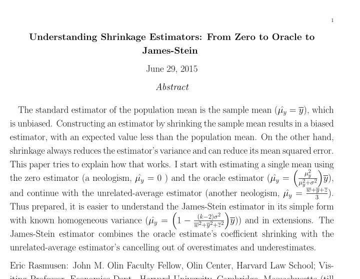
1 Understanding Shrinkage Estimators: From Zero to Oracle to James-Stein June 29, 2015 Abstract The standard estimator of the population mean is the sample mean ( ˆ µ y = y ), which is unbiased. Constructing an estimator by shrinking the sample mean results in a biased estimator, with an expected value less than the population mean. On the other hand, shrinkage always reduces the estimator’s variance and can reduce its mean squared error. This paper tries to explain how that works. I start with estimating a single mean using µ 2 � � y the zero estimator (a neologism, ˆ µ y = 0 ) and the oracle estimator ( ˆ µ y = y ), µ 2 y + σ 2 µ y = w + y + z and continue with the unrelated-average estimator (another neologism, ˆ ). 3 Thus prepared, it is easier to understand the James-Stein estimator in its simple form ( k − 2) σ 2 � � with known homogeneous variance ( ˆ µ y = 1 − y )) and in extensions. The w 2 + y 2 + z 2 James-Stein estimator combines the oracle estimate’s coefficient shrinking with the unrelated-average estimator’s cancelling out of overestimates and underestimates. Eric Rasmusen: John M. Olin Faculty Fellow, Olin Center, Harvard Law School; Vis- iting Professor, Economics Dept., Harvard University, Cambridge, Massachusetts (till

2 Economics and Public Policy, Kelley School of Business, Indiana University.

3 Structure 1. Biased estimators can be “better”. 2. The zero estimator. 3. The seventeen estimator. 4. The oracle estimator. 5. The unrelated-average estimator. 6. The James-Stein estimator with equal and known variances. 7. The positive-part James-Stein estimator. 8. The James-Stein estimator with shrinkage towards the unequal-average. 9. Understanding the James-Stein estimator. 10. The James-Stein estimator with unequal but known variances. 11. The James-Stein estimator with unequal and unknown variances.

4 The James-Stein Estimator W, Y , and Z are normally distributed with unknown means µ w , µ y , and µ z and known identical variances σ 2 . We have one observation on each variable, w, y, z . The sample means are ˆ µ w ( w ) = w, ˆ µ y ( y ) = y , and ˆ µ z ( z ) = y . But for any values that µ w , µ y , and µ z might happen to have, an estimator with lower total mean squared error is the James-Stein estimator which for y is this and for w and z is similar: ( k − 2) σ 2 (1) µ JS,w = w − ˆ w 2 + y 2 + z 2 w, Some questions to think about 1. Why k − 2 instead of k ? 2. Why not shrink towards the unrelated-average mean instead of towards zero? 3. Why not shrink all three towards y instead of towards zero? 4. Why does it not work if σ 2 is different for W, Y, Z and needs to be estimated? 5. Why not use just Y and Z to calculate W’s shrinkage percentage?

5 The Sequence of Thought 1. Hypothesize a value µ r for the true parameter, µ . 2. Pick an estimator of µ as a function of the observed sample: ˆ µ ( y ). 3. Compare µ and ˆ µ ( y ) for the various possible samples we might have give that µ = µ r . Usually we’ll condense this to the mean, variance, and mean squared error µ ( y )) 2 , and E (ˆ µ ( y ) − µ r ) 2 . of the estimator: E ˆ µ ( y ) , E (ˆ µ ( y ) − E ˆ 4. Go back to (1) and try out how the estimator does for another hypothetical value of µ . Keep looping till you’ve covered all possible value of µ .

6 The Zero Estimator The sample mean is ˆ µ y = y Our new estimator, “the zero estimator” is ˆ µ zero = 0 . µ − µ ) 2 (2) MSE (ˆ µ ) = E (ˆ After some algebra, µ ] 2 + E [ˆ µ − µ ] 2 MSE (ˆ µ ) = E [ˆ µ − E ˆ (3) µ ) = E ( Sampling Error ) 2 + Bias 2 MSE (ˆ The sampling error is the distance between ˆ µ and µ that you get because the sample is randomly drawn, different every time you draw it. The bias is the distance between ˆ µ and µ that you’d get if your sample was the entire population, so there was no sampling error. Often one estimator will be better in sampling error and another one in bias. Or, it might be that which estimator is better depends on the true value of µ . Mean squared error weights sampling error and bias equally, but extremes of either of them get more than proportional weight. This will be important.

7 Mean Squared Errors How do our two estimators do in terms of mean square error? The population variance is σ 2 . µ y ) = E [ y − Ey ] 2 + E [ Ey − µ ] 2 MSE (ˆ (4) µ y ) = σ 2 MSE (ˆ and µ zero ) = E [0 − E (0)] 2 + E [ E (0) − µ ] 2 MSE (ˆ (5) µ zero ) = µ 2 MSE (ˆ Thus, y is better than the zero estimator if and only if σ < µ . That makes sense. The zero estimator’s bias is µ , but its variance is zero. By ignoring the data, it escapes sampling error. I If the population variance is high, it is better to give up on using the sample for estimation and just guess zero.

8 The Seventeen Estimator Let me emphasize that the key to the superiority of the zero estimator over y is that variance is high so sampling error is high. The key is not that 0 is a low estimate. The intuition is that there is a tradeoff between bias and sampling error, and so a biased estimator might be best. The “seventeen estimator” is like the zero estimator, except it is defined as ˆ µ 17 = 17. µ seventeen ) = E [17 − E (17)] 2 + E [ E (17) − µ ] 2 MSE (ˆ (6) µ seventeen ) = (17 − µ ) 2 MSE (ˆ The seventeen estimator is better than y if σ > 17 − µ . Thus, it is a good estimator if the variance is big, and a good estimator if the true mean is big and positive. It is not shrinking the estimate from y towards 0 that helps when variance is big: it is making the estimate depend less on the data.

9 III. The Oracle Estimator Let’s next think about shrinkage estimators generally, of which y and the zero esti- mator are the extreme limits. How about an “expansion estimator”, e.g. ˆ µ = 1 . 4 y ? That estimator is biased, plus it depends more on the data, not less, so it will have even bigger sampling error than y . Hence, we can restrict attention to shrinkage estimators. The “oracle estimator” is the best possible (not proved here). It is: � � σ 2 ˆ (7) µ oracle ≡ y − y σ 2 + µ 2 Equation (7) says that if µ is small, we should shrink a bigger percentage. If σ 2 is big, we should shrink a lot. The James-Stein estimator will use that idea.

10 IV. The Unrelated-Average Estimator Suppose we have k = 3 independent estimands, W , Y , and Z . We can still use the sample means, of course— that is to say, use the observed values w , y , and z as our estimator. Or we could use the zero estimator, (0,0,0). But consider “the unrelated average estimator” : the average of the three independent estimands, µ UAE,z ≡ w + y + z µ UAE,w = ˆ ˆ µ UAE,y = ˆ (8) 3 After lots of algebra, � � MSE UAE = σ 2 + 2 ( µ 2 w + µ 2 y + µ 2 z ) − ( µ w µ z + µ w µ y + µ y µ z ) (9) 3 Not bad! In this context, MSE wbar,y,zbar = 3 σ 2 (10) The unrelated-average estimator cuts the sampling error back by 2/3, though at a � � cost of adding bias equal to 2 ( µ 2 w + µ 2 y + µ 2 z ) − ( µ w µ z + µ w µ y + µ y µ z ) . So if the 3 variances are high and the means aren’t too big, we have an improvement over the unbiased estimator.

11 The Unrelated-Average Estimator with Coincidentally Close Es- timands � . Notice what happens if µ w = µ y = µ z = µ . Then MSE UAE = σ 2 + 2 ( µ 2 + 3 � µ 2 + µ 2 ) − ( µ · µ + µ · µ + µ · µ = σ 2 , better than the standard estimator no matter how low the variance is! (unless, of course, σ 2 = 0, in which case the two estimators perform equally well). The closer the three estimands are to each other, the better the unrelated-average estimator works. If they’re even slightly unequal, though, the negative terms in the second part of (10) are outweighed by the positive terms. � If µ w = 3 , µ y = 3 , µ z = 10, for example, the last part of the MSE is 2 (9+9+100) − 3 � � � , and if the variance were only σ 2 = 4 then MSE UAE = 17 = 2 (30 + 9 + 30) 39 3 and MSE wbar,y,zbar = 12. Return to the case of µ w = µ y = µ z , and suppose we know this in advance of getting the data. We have one observation on each of three different independent variables to estimate the population mean when that mean is the same for all three. But that is a problem identical (“isomorphic”, because it maps one to one) to the problem of having three independent observations on one variable.