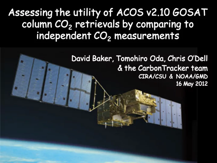
Typical coverage for a sun-synchronous satellite NADIR 4 days - PowerPoint PPT Presentation
Typical coverage for a sun-synchronous satellite NADIR 4 days GLINT 1 day 7 days ~3.5 spacing in longitude ~25 spacing in longitude Outline Satellite data promise a new view: a move from the continental scale to the
Typical coverage for a sun-synchronous satellite NADIR 4 days GLINT 1 day 7 days ~3.5º spacing in longitude ~25º spacing in longitude
Outline Satellite data promise a new view: a move from • the continental scale to the “regional” scale Things needed, first: • Efficient numerical methods for the flux inversion – Understanding of spatial and temporal correlations – of fluxes and column concentrations along orbit Way to remove systematic errors from the – satellite retrievals Here: an attempt at removing systematic • errors from satellite retrievals Is it real or a bias in the satellite retrieval?
GOSAT comparison to CO 2 forward models Compare satellite data to a suite of forward model runs: • CT fluxes TM5 Standard CT release – CT fluxes PCTM ½ °x ⅔ ° – resolution (lat/lon) CSU fluxes PCTM SiB + Doney ocean – CSU fluxes TM5 Just now being run – Sample model at same time/place with same vertical • weighting as the actual measurements Take the obs - model difference • If the differences are all similar, blame it on • retrieval errors
Land, medium-gain 1-to-1 line Land, high-gain Ocean, glint Obs versus model Model versus model (GOSAT vs. CT+PCTM) (CT+TM5 vs. CT+PCTM) Different forward model X CO2 values are closer to each other than any are to the GOSAT-retrieved values Blame GOSAT-model differences on GOSAT retrieval errors (mostly)
Figure courtesy of Chris O’Dell, CSU
Figure courtesy of Chris O’Dell, CSU
Fraction of GOSAT shots passing Chris’ filters Number of shots remaining, 2009-2010: Ocean: 76 K M-Land: 48 K H-land: 73 K Figures courtesy of Chris O’Dell, CSU
Figure courtesy of Chris O’Dell, CSU
Obs – model difference (1 σ ) after fit: 1.55 ppm 1.4 ppm 1.0 ppm Slide courtesy of Chris O’Dell, CSU
Systematic differences (errors?) left after bias correction Aerosol optical depth Latitude “Airmass” = atmospheric path length Signal in O 2 band
x 2 Time-dependence of concentrations on fluxes x 1 x 0 2 1 0 1 x z H H H H 1 1 1 1 1 1 1 0 1 2 x z H H H H 0 2 2 2 2 2 2 0 1 2 3 x z H H H H 3 3 3 3 3 3 1 2 3 4 x z H H H H 4 4 4 4 4 4 2 3 4 5 x z H H H H 5 5 5 5 5 5 H M 4 M 3 M 2 M 1 x z H H H H M 1 M 1 1 1 1 1 M M M M M 3 M 2 M 1 M x z H H H H M M M M M M fluxes Transport basis functions concentrations
4D-Var: NWP vs. carbon flux estimation prediction Solve for I.C.s over multiple NWP short windows (6 hours): driven by the need to x 0 update predictions x 0 … … x 0 assimilation x 0 window Carbon Solve for B.C.s (fluxes) and I.C.s over fluxes long window (1 year +): retrospective … … u I-1 x 0 u 0 u 1
4-D Var Iterative Optimization Procedure 0 x 0 Forward Forward Estimated “True” ° 1 Transport Transport Fluxes Fluxes 2 Modeled “True” ° Concentrations Concentrations x 1 Measurement Measurement ° x 2 Sampling Sampling Modeled “True” Measurements Measurements Assumed /(Error) 2 Measurement 3 Errors x 3 ° Weighted Measurement Residuals Flux Adjoint Update Transport Adjoint Fluxes = Minimum of cost function J
CO 2 flux estimation approach using GOSAT X CO2 Variational carbon data assimilation system • Optimize weekly CO 2 fluxes for 2010 at 4½°x6° (lat/lon) • Prior fluxes, a CarbonTracker “projection” (Jacobson): • fossil fuel from preliminary 2010 statistics (CDIAC) – “climatological” fluxes for land biosphere and ocean – (average of 2000-2009 values from CT 2010) NOT optimized against in situ data for 2010 – PCTM off-line atmospheric transport model, driven by • GEOS5 analyzed meteorology fields CT fluxes run thru at ½°x ⅔ ° (lat/lon) to get prior [CO2] – Flux corrections estimated at 4½°x6° (lat/lon) –
4DVar flux inversion cases Seven flux inversions cases for 2010 using: NOAA in situ : 62 weekly flask sites, 4 continuous • sites, 8 tall towers (daily) TCCON columns, 14 sites • Screened ACOS ver. 2.9 GOSAT X CO2 : • No bias correction – a separate 3-parameter bias correction for ocean and high- – and medium-gain land data Three bias corrections of Wunch, et al (2011) –
4DVar CO 2 Flux Estimates w/ ACOS v.2.9 GOSAT X CO2 = Post. - Prior Post. w/ GOSAT data Projected CT Prior Δ Apr-Jun 2010 Jul-Sep 2010 Full year 2010 10 -8 [kgCO 2 m -2 s -1 ]
CO 2 flux corrections to the CT-PCTM prior [10 -8 kgCO 2 m -2 s -1 ] when assimilating only: ACOS v2.9 GOSAT NOAA H-Land, M-Land, & Ocean H-Land & Ocean TCCON in situ Wunch bias corr., H-L only No bias correction 3-param. bias corr. JFM DJF AMJ MAM JAS JJA OND SON Ann ANN
Evaluation of a posteriori CO 2 fields against independent data 1 σ error [ppm] between optimized model and TCCON (in 2-hr bins) [ppm] Prior 1.30 Prior 1.307 in situ GOSAT, H+M+Ocn, no bias corr. 1.204 1.25 GOSAT, H+M+Ocn, 3-param. “ 1.172 GOSAT, no corr 1.20 GOSAT, H+Ocn, Wunch #1 “ 1.219 GOSAT, 3-param. GOSAT, H+Ocn, Wunch #2 “ 1.219 1.15 GOSAT, H+Ocn, Wunch #3 “ 1.213 1.10 NOAA in situ 1.268 TCCON 1.054 1.05 TCCON
Figure 3 from Chevallier, et al (2011) TCCON inversion paper. Next: make a similar plot for inversions / data comparisons using: • ACOS GOSAT XCO2 • NOAA surface in situ data • NOAA routine aircraft profiles • TCCON XCO2 • HIPPO, AIRS, TES, AirCore, etc
EnKF & 4DVar KF sliding flux window with N times fluxes in it EnKF Measurement span 4DVar Computational work: Backward propagation of • N times *N ens for EnKF (in parallel) information: • 4*N iter for 4DVar (serial) For EnKF, depends on time width of window – shorter Columns in C, where P=CC T : spans give poorer constraints N ens for EnKF at larger time/space scales 2*N iter for 4DVar
Recommend
More recommend
Explore More Topics
Stay informed with curated content and fresh updates.

