Two-stage Benchmarking of Time-Series Models for Small Area - PowerPoint PPT Presentation

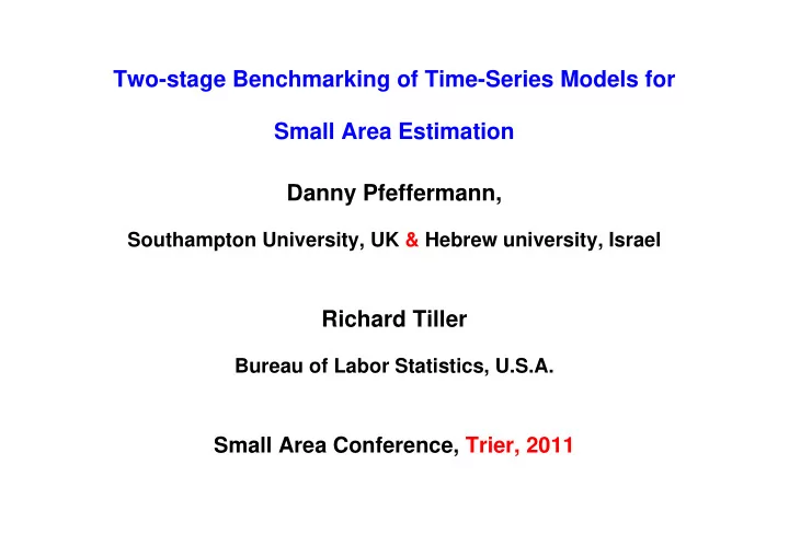
Two-stage Benchmarking of Time-Series Models for Small Area Estimation Danny Pfeffermann, Southampton University, UK & Hebrew university, Israel Richard Tiller Bureau of Labor Statistics, U.S.A. Small Area Conference, Trier, 2011

What is benchmarking? = 1,2,..., Areas d D Y - target characteristic in area d at time t , , = dt 1,2,... Time t y - direct survey estimate, dt ˆ model Y - estimate obtained under a model. dt Benchmarking: modify model based estimates to satisfy : ∑ = ∑ D ˆ = D model t = , ,... ( 1 2 ; B known , e.g., ). d b Y B B b y = dt dt t t t = dt dt 1 1 d b fixed coefficients (relative size, scale factors ,… ). dt ∑ D B sufficiently close to true value Condition: . d b Y t = dt dt 1 ˆ model Y not necessarily a linear estimator. dt 2

Problem considered in present presentation Develop a two-stage benchmarking procedure for hierarchical time series models fitted to survey estimates. First stage: benchmark concurrent model-based estimators at higher level of hierarchy to reliable aggregate of corresponding survey estimates. Second stage: benchmark concurrent model-based estimates at lower level of hierarchy to first stage benchmarked estimate of higher level to which they belong. 3

Example: Labour Force estimates in the U.S.A 4

Why benchmark? 1- Time series models reflect historical behavior of the series. Slow in adapting to changes ⇒ benchmarking provides some protection against abrupt changes affecting the areas in a given hierarchy. 2- The published benchmarked estimates at each level sum up to the published estimate at the higher level. Required by official statistical bureaus. 3- Another way of ‘borrowing strength’ across areas. 5

Why not benchmark second level areas in one step? 1- May not be feasible in a real time production system : For U.S.A.-CPS our proposed procedure requires joint modeling of all the areas that need to be benchmarked, ⇒ state-space model of order 700 . 2- Delay in processing data for one second level area could hold up all the area estimates. 3- When 1 st – level hierarchy composed of homogeneous 2 nd level areas, benchmarking more effectively tailored to 1 st – level characteristics. 6

Apply cross-sectional benchmarking at every time t? Pro-rata (ratio) benchmarking , = ∑ ∑ D D ˆ = ˆ × Β ˆ bmk model model / ) ; . Y Y b Y B b y R , = = d d k k d d 1 1 k d Limitations: 1- Adjusts all the small area model-based estimates exactly the same way, irrespective of their precision, 2- Benchmarked estimates not consistent: if sample size in area d increases but sample sizes in other areas unchanged, ˆ bmk Y . Y R does not converge to true population value d d, 7

Limitations of independent pro-rata benchmarking (cont.) 3- Does not lend itself to simple variance estimation. 4- If applied independently at every time point ⇒ ignores inherent time series relationships between the benchmarks = ∑ ⇒ may add extra roughness to benchmarked D B b y t = dt dt 1 d estimates and the corresponding estimated trend. Possibly similar problem with all cross-sectional benchmarking procedures when applied to a time series. 8

Additive cross-sectional benchmarking ∑ ∑ ∑ ˆ = ˆ + D − D ˆ D = model a model 1 . bmk ( ) ; Y Y b y b Y d b a A d , d d = k k = k k = d d 1 1 1 k k Coefficients { a } measure precision (next slide) ; distribute d difference between benchmark and aggregate of model- based estimates between the areas. → ⇒ ˆ A → ˆ → ⇒ consistent . bmk model 0 If a Y Y Y , d n d d d →∞ d ˆ − = ⇒ Area d accurate estimate bmk Plim( ) 0 Bad news? Y y A , d d →∞ n d not contributing to benchmarking in other areas. ˆ bmk ‘ Easy ’ to estimate variance of A . Y , d 9

Examples of additive cross-sectional benchmarking ∑ 2 D − ˆ φ bmk ( ) Wang et al . (2008) minimize under F-H E Y Y d A , = d d 1 d ∑ ∑ ∑ − − D = D ˆ = ϕ D ϕ � 1 1 2 bmk A . Sol : / s.t. . b y b Y a b b , = d d = d d d d d = k k 1 1 1 d d k φ } represent precision of direct or model-based estimators. { d − = ˆ → Battese et al . 1988 . φ model 1 [ ( )] Var Y d d ∑ = D − ˆ ˆ → Pfeffermann & Barnard 1991 . φ model model 1 [cov( , )] b Y Y d d d = k 1 k − = → Isaki et al . 2000 . φ 1 [ ( )] Var y d d In practice, model parameters replaced by estimates. 10

Examples of additive cross-sectional benchmark. (cont.) ∑ 2 D − ˆ φ [ | data ] bmk Datta et al . (2011) minimize ( ) and E Y Y d A = d d , 1 d = ˆ model | data . ( ) obtain solution of Wang et al ., with Y E Y d d Solution general - not restricted to particular model. You and Rao (2002) propose “self benchmarked” estimators for unit-level model by modifying the estimator of β . Approach applied by Wang et al . (2008) to area-lave model. Ugarte et al . (2009) benchmark the BLUP under unit-level model to synthetic estimator for all areas under regression model with heterogeneous variances. 11

First-stage time series benchmarking Pfeffermann & Tiller (2006) consider the following model for unemployment census division series obtained from CPS . ′ = ′ … = ( , , ) y y y ( ,..., ) Let = true division totals , = Y Y Y 1 1 t t Dt t t Dt ′ = … ( , , ) e e e direct estimates , = sampling errors . 1 t t Dt ( ) ′ = + = = = σ σ … ; , Σ Diag 2 2 ( ) 0 [ , , ] . y Y e E e E e e τ τ τ τ t 1, , , , t t t t t t D t Division sampling errors independent between divisions but highly auto-correlated within a division and heteroscedastic. ( 4 in , 8 out , 4 in rotation pattern) 12

Time series model for division d Y assumed to evolve independently between divisions Totals dt according to basic structural model ( BSM, Harvey 1989 ). Model accounts for stochastic trend , stochastically varying seasonal effects and random irregular terms . ′ = α α = α + η ; Y z T Model written : . ( state-space ) − , 1 dt dt dt dt d d t dt η mutually independent white noise, ( η η ′ = ) E Q Errors . dt dt dt d ARIMA , regression with random coefficients and unit & area level models can all be expressed in state-space form. 13

Combining the separate division models ′ = + = α + = ( measurement eq. ) ; ( ,..., ) , y Y e Z e y y y 1 D t t t t t t t t t � ′ ′ ′ α = α + η α = α α , ( ,..., ) T ( state eq. ) ; − 1 D 1 t t t t t t , � ′ = Ι ⊗ = Ι ⊗ ; ⊗ - block diagonal Z z T T t D dt D d ( ) ( ) ( ) ′ ′ η = ηη = =Ι ⊗ η η = τ ≠ , , , 0 0 . E E Q Q E t τ t t t D d t Benchmark constraints: MODEL ∑ ∑ ∑ ′ D = D α = D , t = 1,2,... b y b z b Y = = = dt dt dt dt dt dt dt 1 1 1 d d d ∑ ∑ ∑ D D D ′ = b z α + d=1 b e . But in truth, b y dt dt = dt dt = dt dt dt 1 1 d d 14

Adding benchmark equations to model ∑ ∑ ∑ ′ D D D = α + Add to measurement eq. b y b z b e = = = dt dt dt dt dt dt dt 1 1 1 d d d ′ ∑ � ′ D = α + = � � ; � ( ) y Z e y y b y , , t t t t t t = dt dt 1 d ′ ( ) ⎡ ⎤ Z ∑ � ′ D = = � t , Z ⎢ ⎥ e e b e . ′ ′ , t … t t = dt dt 1 ⎣ 1 , , ⎦ d b z b z 1 t t Dt Dt � α = α + η T State equations unchanged . − 1 t t t 15

Set up random coefficients regression model � � ⎛ ⎞ ⎛ ⎞ α ⎛ ⎞ bmk bmk I T u � − = α + − = α − α � , 1 | 1 bmk bmk t t t ⎜ ⎟ ⎜ ⎟ ; ⎜ ⎟ u T � − − � Z t t t | 1 t 1 t � y ⎝ ⎠ ⎝ ⎠ ⎝ ⎠ e t t t ⎡ ⎤ Σ bmk ⎡ ⎤ ⎛ ⎞ = C bmk P h bmk u � − � E e e ′ t Σ = = ⎢ | 1 � � − t t = tt tt ⎢ ⎥ | 1 V ( ) t t . ; ⎜ ⎟ ⎥ Var ′ t ′ tt t t � � ⎣ ⎦ h v ⎢ bmk ⎥ ⎝ ⎠ e C Σ ⎣ ⎦ tt tt t t tt ∑ ∑ D D = = ( , ) ( ) ; . h Cov e b e v Var b e tt t = dt dt tt = dt dt 1 1 d d = ∑ − ′ 1 = t τ t → linear combination of � Σ bmk bmk ( ) C E u e D τ − | 1 τ = t t t t 1 covariance matrices of sampling errors. 16

Imposing benchmark constraints ∑ ∑ ⇔ ∑ D ′ D D = b z α d=1 b e = 0 Impose , when b y dt dt = = dt dt dt dt dt 1 1 d d estimating the state vector under RCR model. Define , ⎡ ⎤ bmk C bmk P � e ′ ′ E e e ′ − = Σ = − ′ � � � = � t, 0 � | 1 tt bmk bmk = ⎢ ( ,0) ( ) ⎥ , , ( ) , e C E u e V 0 0 0 0 0 0 , , , , t t tt t t , | 1 , 0 t t t t ′ , � t Σ bmk ⎢ ⎥ C ⎣ ⎦ t, 0 0 tt , − 1 � � ⎡ Ι ⎤ ⎛ ⎞ ⎛ ⎞ α bmk T � � � � ′ ′ = Ι − Ι − − → ‘standard’ GLS . � bmk α 1 1 1 t ⎢ ( , ) ⎥ ( , ) ⎜ ⎟ Z V ⎜ ⎟ Z V � t 0 0 , , t t t t � ⎝ ⎠ Z ⎣ ⎦ ⎝ ⎠ y t t z ′ Benchmarked predictor for division d : ˆ bmk = � bmk α . Y dt dt dt 17