Two-photon exchange calculations versus data Oleksandr Tomalak - PowerPoint PPT Presentation

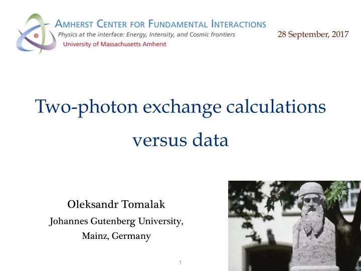
28 September, 2017 Two-photon exchange calculations versus data Oleksandr Tomalak Johannes Gutenberg University, Mainz, Germany 1

Scattering experiments and 2 Ɣ - 2 Ɣ is not among standard radiative corrections σ exp ≡ σ 1 γ (1 + δ rad + δ soft + δ 2 γ ) - charge radius insensitive to 2 Ɣ model - magnetic radius depends on 2 Ɣ model J. C. Bernauer et al. (2014) 2

Scattering experiments and 2 Ɣ - 2 Ɣ is not among standard radiative corrections σ exp ≡ σ 1 γ (1 + δ rad + δ soft + δ 2 γ ) - charge radius insensitive to 2 Ɣ model - magnetic radius depends on 2 Ɣ model J. C. Bernauer et al. (2014) magnetic form factor - 2 % systematic deviation MAMI vs. world data 3

µH hyperfine splitting and 2 Ɣ 1 S HFS in H µ PSI, J-PARC, RIKEN-RAL 1 ppm accuracy R. Pohl et al. (2016) - leading theoretical uncertainty: 213 ppm from 2 Ɣ , 109 ppm from 2 Ɣ C. Carlson, V. Nazaryan, K. Griffioen (2011) Cl. Peset and A. Pineda (2017) - HFS in terms of forward lepton-proton scattering amplitudes O. Tomalak (2017) - traditional decomposition: ∆ HFS = ∆ Z + ∆ R + ∆ pol Zemach term polarizability recoil correction G E , G M F 2 , g 1 , g 2 G E , G M - A1@MAMI fit allows to quantify 2 Ɣ uncertainty J. C. Bernauer et al. (2014) - magnetic radius, form factors and spin structure are important 4

Zemach contribution - Zemach correction expanding form factors ∞ ! � Q 2 � � Q 2 � M + r 2 E r 2 G M G E ✓ ◆ ∆ Z = 8 α m r Z d Q + 4 α m r Q 0 − r 2 E − r 2 18 Q 2 M − 1 0 Q 2 µ P 3 π π Q 0 - dependence on splitting: consistency check dependence on Q 2 dependence on Q 2 0 − 7.3 0 Δ Z , Q 0 = 0 − 7.3 Δ Z , Q 0 = 0 10 3 ×Δ Z 10 3 ×Δ Z − 7.4 − 7.4 ✓ − 7.5 r E from ep scattering r E from μ H − 7.5 0 0.01 0.02 0.03 0.04 0.05 0.06 0 0.01 0.02 0.03 0.04 0.05 0.06 Q 2 0 , GeV 2 Q 2 0 , GeV 2 O. Tomalak (2017) - 95 ppm change for μ H and ep radii with Q 0 = 0.2 GeV - 3 times more precise: 140 ppm → 49 ppm - magnetic radius is important 5

Hyperfine splitting and 2 Ɣ eH - compare with precise 1S HFS from eH achieved accuracy in 70th: 10 -12 − 34 − 33 − 32 − 31 Δ HFS , ppm Δ pol , Faustov et al. R E from ep, eH Δ Z + Δ R , Bodwin et al. R E from μ H Carlson et al. 1S HFS in eH - dispersive evaluation and phenomenological extractions agree 6

Hyperfine splitting and 2 Ɣ eH - compare with precise 1S HFS from eH achieved accuracy in 70th: 10 -12 − 34 − 33 − 32 − 31 Δ HFS , ppm Δ pol , Faustov et al. R E from ep, eH Δ Z + Δ R , Bodwin et al. R E from μ H Carlson et al. 1S HFS in eH - dispersive evaluation and phenomenological extractions agree 7

Hyperfine splitting and 2 Ɣ eH - compare with precise 1S HFS from eH achieved accuracy in 70th: 10 -12 − 34 − 33 − 32 − 31 Δ HFS , ppm Δ pol , Faustov et al. R E from ep, eH Δ Z + Δ R , Bodwin et al. R E from μ H Carlson et al. 1S HFS in eH μ H - exploit eH HFS measurements scaled by a reduced mass m r ∆ ( µ H) = m r ( m µ ) m r ( m e ) ∆ (eH)+ ∆ HFS ( m µ ) − m r ( m µ ) m r ( m e ) ∆ HFS ( m e ) − 7.0 − 6.5 − 6.0 10 3 Δ HFS with 1S HFS in eH Hagelstein et al. Carlson et al. - uncertainty: 100 ppm → 16 ppm !!! R E from ep, eH Peset et al. Martynenko et al. R E from μ H 2S HFS in μ H, CREMA Pachucki - dispersive evaluation and phenomenological extractions agree 8

Hyperfine splitting and 2 Ɣ eH - compare with precise 1S HFS from eH achieved accuracy in 70th: 10 -12 − 34 − 33 − 32 − 31 Δ HFS , ppm Δ pol , Faustov et al. R E from ep, eH Δ Z + Δ R , Bodwin et al. R E from μ H Carlson et al. 1S HFS in eH μ H - exploit eH HFS measurements scaled by a reduced mass m r ∆ ( µ H) = m r ( m µ ) m r ( m e ) ∆ (eH)+ ∆ HFS ( m µ ) − m r ( m µ ) m r ( m e ) ∆ HFS ( m e ) − 7.0 − 6.5 − 6.0 10 3 Δ HFS with 1S HFS in eH Hagelstein et al. Carlson et al. - uncertainty: 100 ppm → 16 ppm !!! R E from ep, eH Peset et al. Martynenko et al. R E from μ H 2S HFS in μ H, CREMA Pachucki - dispersive evaluation and phenomenological extractions agree 9

Elastic lepton-proton scattering momentum transfer Q 2 = − ( k − k 0 ) 2 photon polarization l ( k ) l ( k 0 ) parameter ε crossing-symmetric variable p 0 forward scattering p ν = ( k, p + p 0 ) ε → 1 2 - leading 2 Ɣ contribution: interference term 2 l l l T 1 γ < T 2 γ l 2 P spin δ 2 γ = γ γ γ P | T 1 γ | 2 spin p p p p - 2 Ɣ correction to cross section is given by amplitudes real parts 10

Elastic lepton-proton scattering l ( k ) l ( k 0 ) K = k + k 0 P = p + p 0 2 2 p 0 p - electron-proton scattering: 3 structure amplitudes ˆ T non − flip = e 2 N ( G M ( ν , Q 2 ) γ µ − F 2 ( ν , Q 2 ) P µ KP µ Q 2 ¯ l γ µ l · ¯ M + F 3 ( ν , Q 2 ) M 2 ) N P.A.M. Guichon and M. Vanderhaeghen (2003) - muon-proton scattering: add helicity-flip amplitudes ˆ T flip = e 2 M ) N + e 2 m K m ¯ ll · ¯ M F 6 ( ν , Q 2 )¯ l γ 5 l · ¯ N ( F 4 ( ν , Q 2 ) + F 5 ( ν , Q 2 ) N γ 5 N Q 2 Q 2 M M. Gorchtein, P.A.M. Guichon and M. Vanderhaeghen (2004) - 2 Ɣ correction to cross section is given by amplitudes real parts 11

non-forward scattering at low momentum transfer l 0 l γ γ p 0 p photoproduction vertex or Compton tensor box diagram assumption about the vertex 12

non-forward scattering at low momentum transfer l 0 l γ γ p 0 p photoproduction vertex or Compton tensor box diagram dispersion relations assumption about the vertex based on on-shell information 13

non-forward scattering proton state l 0 l γ γ p 0 p Dirac and Pauli form factors box diagram dispersion relations assumption about the vertex based on on-shell information Blunden, Melnitchouk and Tjon (2003) Borisyuk and Kobushkin (2008), O. T. and M. Vanderhaeghen (2014) 14

near-forward scattering forward scattering account for all inelastic 2 Ɣ l 0 l l l γ γ γ γ p 0 p p p 15

Low-Q 2 inelastic 2 Ɣ correction (e - p) l 0 - 2 Ɣ blob: near-forward virtual Compton scattering l Feshbach inelastic elastic γ γ p 0 Q 2 + b Q 2 ln Q 2 + c Q 2 ln 2 Q 2 p p δ 2 γ ∼ a R. W. Brown (1970), M. Gorchtein (2013), O. T. and M. Vanderhaeghen (2014) unpolarized proton structure M. E. Christy, P. E. Bosted (2010) Z d ν γ d Q 2 ( w 1 ( ν γ , Q 2 ) · F 1 ( ν γ , Q 2 ) + w 2 ( ν γ , Q 2 ) · F 2 ( ν γ , Q 2 )) δ 2 γ = 1.5 A1@MAMI Q 2 = 0 . 25 GeV 2 A1@MAMI 1.5 Feshbach Feshbach box diagram model box diagram model 1.0 total 2 γ total 2 γ δ 2 γ , % δ 2 γ , % 1.0 0.5 0.5 Q 2 = 0 . 05 GeV 2 0 0.1 0.2 0.3 0.4 0.5 0.6 0.7 0.8 0.9 1.0 0.1 0.2 0.3 0.4 0.5 0.6 0.7 0.8 0.9 1.0 ε ε O. T. and M. Vanderhaeghen (2016) r E extraction ✓ - 2 Ɣ at large agrees with empirical fit ε 16

Scattering experiments and 2 Ɣ - charge radius extractions: eH, eD spectroscopy ep scattering μ H, μ D spectroscopy μ p scattering ???? - μ p elastic scattering is planned by MUSE@PSI(2018-19) measure with both electron/muon charges - 2 Ɣ correction in MUSE ? 17

MUSE@PSI (2018-19) estimates ( - p) µ - proton box diagram model + inelastic 2 Ɣ 1.0 box diagram model, μ - p 1.0 total, μ - p total, e - p δ 2 γ , % δ 2 γ , % 0.5 0.5 k = 115 MeV k = 210 MeV 0 0 0 0.005 0.010 0.015 0.020 0.025 0 0.02 0.04 0.06 0.08 Q 2 , GeV 2 Q 2 , GeV 2 O. T. and M. Vanderhaeghen (2014, 2016) 18

MUSE@PSI (2018-19) estimates ( - p) µ - proton box diagram model + inelastic 2 Ɣ 1.0 box diagram model, μ - p 1.0 total, μ - p total, e - p δ 2 γ , % δ 2 γ , % 0.5 0.5 k = 115 MeV k = 210 MeV 0 0 0 0.005 0.010 0.015 0.020 0.025 0 0.02 0.04 0.06 0.08 Q 2 , GeV 2 Q 2 , GeV 2 O. T. and M. Vanderhaeghen (2014, 2016) - expected muon over electron ratio small inelastic 2 Ɣ small 2 Ɣ uncertainty - MUSE can test r E in one charge channel K. Mesick talk (PAVI 2014), MUSE TDR (2016) 19

near-forward scattering dispersion relations (large ) (arbitrary ) ε ε l 0 l 0 l l γ γ γ γ p 0 p 0 p p X X = p + π N p + all inelastic 20

Fixed-Q 2 dispersion relation framework on-shell 1 Ɣ amplitudes 2 Ɣ prediction cross section correction experimental data = F ( ν 0 + i 0) Z 1 < F ( ν ) = 2 ν unitarity d ν 0 π P ν 0 2 � ν 2 ν min disp. rel. 2 Ɣ imaginary parts 2 Ɣ real parts 21

Mandelstam plot (ep) Q 2 , GeV 2 s = ( M + m π ) 2 1.0 s = M 2 0.8 0.6 unitarity relations 0.4 work in physical region 0.2 ν , GeV 2 − 0.2 0.2 0.4 elastic threshold inelastic threshold - proton intermediate state is outside physical region for Q 2 > 0 - π N intermediate state is outside physical region for Q 2 > 0.064 GeV 2 O. T. and M. Vanderhaeghen (2014) 22

Analytical continuation. Elastic state - contour deformation method: O. T. and M. Vanderhaeghen (2014), Blunden and Melnitchouk (2017) angular integration deform integration contour Z d Ω to integration on curve keeping poles inside in complex plane going to unph. region unphysical physical e − µ − box - analytical continuation 0.01 = G M reproduces results ✓ in unphysical region 0 Q 2 = 0 . 1 GeV 2 ν ph − 0.02 0 0.02 0.04 0.06 0.08 ν , GeV 2 - central value: form factor fit of A1@MAMI (2014) - uncertainty: difference to 2 Ɣ with dipole form factors 23