Turing Machines (TM) Deterministic Turing Machine (DTM) - PowerPoint PPT Presentation
Turing Machines (TM) Deterministic Turing Machine (DTM) Nondeterministic Turing Machine (NDTM) 1 Deterministic Turing Machine (DTM) .. .. B B 0 1 1 0 0 B B Finite Control Two-way, infinite tape, broken into
Turing Machines (TM) • Deterministic Turing Machine (DTM) • Nondeterministic Turing Machine (NDTM) 1
Deterministic Turing Machine (DTM) …….. …….. B B 0 1 1 0 0 B B Finite Control • Two-way, infinite tape, broken into cells, each containing one symbol. • Two-way, read/write tape head. • Finite control, i.e., a program, containing the position of the read head, current symbol being scanned, and the current state. • An input string is placed on the tape, padded to the left and right infinitely with blanks, read/write head is positioned at the left end of input string. • In one move, depending on the current state and symbol being scanned, the TM: – changes state – prints a symbol over the cell being scanned, and – moves its’ tape head one cell left or right. 2
Formal Definition of a DTM • A DTM is a seven-tuple: M = (Q, Σ, Γ, δ, q 0 , B, F) Q A finite set of states Γ A finite tape alphabet A distinguished blank symbol, which is in Γ B Σ A finite input alphabet, which is a subset of Γ– {B} q 0 The initial/starting state, q 0 is in Q F A set of final/accepting states, which is a subset of Q δ A next-move function, which is a mapping (i.e., may be undefined) form Q x Γ –> Q x Γ x {L,R} Intuitively, δ(q,s) specifies the next state, symbol to be written, and the direction of tape head movement by M after reading symbol s while in state q. 3
• Example #1: {w | w is in {0,1}* and w ends with a 0} 0 00 10 10110 Not ε Q = {q 0 , q 1 , q 2 } Γ = {0, 1, B} Σ = {0, 1} F = {q 2 } δ: 0 1 B q 0 (q 0 , 0, R) (q 0 , 1, R) (q 1 , B, L) q 1 (q 2 , 0, R) - - q 2 - - - – q 0 is the “scan right” state – q 1 is the verify 0 state 4
• Example #1: {w | w is in {0,1}* and w ends with a 0} 0 1 B q 0 (q 0 , 0, R) (q 0 , 1, R) (q 1 , B, L) q 1 (q 2 , 0, R) - - q 2 - - - • Sample Computation: (on 0010) q 0 0010 | — 0q 0 010 | — 00q 0 10 | — 001q 0 0 | — 0010q 0 | — 001q 1 0 | — 0010q 2 5
Example #2: {0 n 1 n | n >= 1} • 0 1 X Y B q 0 (q 1 , X, R) - - (q 3 , Y, R) - q 1 (q 1 , 0, R) (q 2 , Y, L) - (q 1 , Y, R) - q 2 (q 2 , 0, L) - (q 0 , X, R) (q 2 , Y, L) - q 3 - - - (q 3 , Y, R) (q 4 , B, R) q 4 - - - - - • Sample Computation: (on 0011) q 0 0011 | — Xq 1 011 | — X0q 1 11 | — Xq 2 0Y1 | — q 2 X0Y1 | — Xq 0 0Y1 | — XXq 1 Y1 | — XXYq 1 1 | — XXq 2 YY | — Xq 2 XYY | — XXq 0 YY | — XXYq 3 Y | — XXYYq 3 | — XXYYBq 4 6
Example #2: {0 n 1 n | n >= 1} • 0 1 X Y B q 0 (q 1 , X, R) - - (q 3 , Y, R) - q 1 (q 1 , 0, R) (q 2 , Y, L) - (q 1 , Y, R) - q 2 (q 2 , 0, L) - (q 0 , X, R) (q 2 , Y, L) - q 3 - - - (q 3 , Y, R) (q 4 , B, R) q 4 - - - - - – The TM basically matches up 0’s and 1’s – q 0 is the “check off a zero” state – q 1 is the “scan right, find and check off a matching 1” state – q 2 is the “scan left” state – q 3 is the “ verify no more ones” state – q 4 is the final state • Other Examples: 000111 00 11 001 011 010 110 7
• Definition: Let M = (Q, Σ, Г, δ, q 0 , B, F) be a TM. The language accepted by M , denoted L(M), is the set {w | w is in Σ* and w is accepted by M} 8
• What kinds of things can TMs do? – Accept languages (as above) – Simulate DFAs, NFAs and PDAs – Compute functions and operators (+, *, etc) – Have subroutines, pass parameters – Simulate arbitrary computer programs • Exercises: Construct a DTM for each of the following. – {w | w is in {0,1}* and w ends in 00} – {w | w is in {0,1}* and w contains at least 2 0’s} – {w | w is in {0,1}* and w contains at least one 0 and one 1} – {w | w is in {0,1}* and w contains at least one occurrence of the substring 00} – A TM that adds 1 to a given binary number – Suppose the input to a Turing machine consists of two n-bit binary numbers separated by a # character. Give a deterministic Turing machine that will determine if the first binary number is larger than the second. Note that the turning machine should output 1 to the right of the second number if the answer is yes, and a 0 if the answer is no. 9
Be Careful! • Note that, just like a computer program, a TM can contain an infinite loop: 0 1 B q 0 (q 0 , 0, R) (q 0 , 1, R) (q 0 , B, R) • This is somewhat equivalent to: while (true) ; • As with more general programs, more complicated TM infinite loops can occur. 10
TM Computations • In summary, given an arbitrary Turing machine M, and a string x, there are three possible types of computations: – M terminates in a final state, in which case we say x is accepted and in L(M). – M terminates in a non-final state, in which case we say x is not accepted and is not in L(M). – M goes into an infinite loop, in which case we say x is not accepted and is not in L(M). • Stated another way, given an arbitrary Turing machine M, and a string x: – If x is in L(M) then M will halt in a final state. – If x is not in L(M) then M may enter an infinite loop, or halt in a non-final state. 11
TMs as a General Model of Computation • Questions: – How difficult would it be to simulate an arbitrary TM with a computer program? – How difficult would it be to simulate an arbitrary computer program with a TM? • TMs Model General Purpose Computers: – If a TM can do it, so can a GP computer – If a GP computer can do it, then so can a TM 12
• More formally, this is codified in the Church-Turing Thesis: There is an “effective procedure” for solving a problem if and only if there is a TM that halts for all inputs and solves the problem. • Informally, the notion of an “effective procedure” is intended to represent a program that a real, general purpose computer could execute: – Finitely describable – Well defined, discrete, “mechanical” steps – Always terminates • TMs formalize the above notion, i.e., the computing capability of a general purpose computer. • Other models, such as DFAs and PDAs do not model all effective procedures or computable functions, but only a subset. 13
Modifications of the Basic TM Model • There are many other computing models, but all are equivalent to or subsumed by TMs. There is no more powerful machine (Technically not proven). • Other (Extended) TM Models: – One-way infinite tapes – Multiple tapes and tape heads – Non-Deterministic TMs – Multi-Dimensional TMs (n-dimensional tape) – Multi-Heads – Multiple tracks All of these extensions are “equivalent” to the basic TM model * 14 *In terms of the languages accepted, but not necessarily in terms of performance.
Recommend
More recommend
Explore More Topics
Stay informed with curated content and fresh updates.

![Turing Machines A more powerful computation model than a PDA ? [Section 9.1] Turing Machines](https://c.sambuz.com/785218/turing-machines-s.webp)
