Turing Machines 9-0 Turing Machines Now for a machine - PDF document
Griffith University 3130CIT Theory of Computation (Based on slides by Harald Sndergaard of The University of Melbourne) Turing Machines 9-0 Turing Machines Now for a machine model of much greater power. A
✬ ✩ Griffith University 3130CIT Theory of Computation (Based on slides by Harald Søndergaard of The University of Melbourne) Turing Machines ✫ ✪ 9-0
✬ ✩ Turing Machines Now for a machine model of much greater power. A Turing machine has an infinite tape through which it takes its input and performs its computations. state control tape head b a a infinite tape � � � � Unlike a finite automaton it can • both read from and write to the tape, and • move either left or right over the tape. The tape is infinite. The machine has both accept and reject states, in which it accepts/rejects irrespective of where its ✫ tape head is. ✪ 9-1
✬ ✩ Turing Machines Formally A Turing machine is a 7-tuple M = ( Q, Σ , Γ , δ, q 0 , q a , q r ) where • Q is a finite set of states, • Γ is a finite tape alphabet, which includes the blank character, � � , • Σ ⊆ Γ \ { � � } is the input alphabet, • δ : Q × Γ → Q × Γ × { L, R } is the transition function, • q 0 is the initial state, • q a is the accept state, and • q r ( � = q a ) is the reject state. ✫ ✪ 9-2
✬ ✩ The Transition Function A transition δ ( q i , x ) = ( q j , y, d ) depends on two things 1. current state q i , and 2. current symbol x under the tape head It consists of three actions 1. change state to q j , 2. over-write tape symbol x by y , and 3. move the tape head in direction d . We can have a graphical notation for Turing machines similar to that for finite automata. On an arrow from q i to q j we write • x → d when δ ( q i , x ) = ( q j , x, d ), and • x → y, d when δ ( q i , x ) = ( q j , y, d ) , y � = x . ✫ ✪ 9-3
� � � � ✬ ✩ Example Turing Machine b → R � ���� ���� ���� ���� ���� ���� a → R � a → R � q 0 q 1 q a � � b → R � � � � � → R � � � � → R � � � ���� ���� � q r This machines recognises the regular language ( a ∪ b ) ∗ aa ( a ∪ b ) ∗ . We can leave q r out with the understanding that transitions that are not specified go to q r . ✫ ✪ 9-4
✬ ✩ Turing Machine Configurations We write uqv for this configuration: blank u v q On input aba , the example machine goes through these configurations: ǫq 0 aba (or just q 0 aba ) ⊢ aq 1 ba ⊢ abq 0 a ⊢ abaq 1 � � ⊢ aba � � q r We read the relation ‘ ⊢ ’ as “yields”. ✫ ✪ 9-5
✬ ✩ Computations Formally For all q i , q j ∈ Q , a, b, c ∈ Γ, and u, v ∈ Γ ∗ , we have uq i bv ⊢ ucq j v if δ ( q i , b ) = ( q j , c, R ) q i bv ⊢ q j cv if δ ( q i , b ) = ( q j , c, L ) uaq i bv ⊢ uq j acv if δ ( q i , b ) = ( q j , c, L ) The start configuration of M on input w is q 0 w . M accepts w iff there is a sequence of configurations C 1 , C 2 , . . . , C k such that 1. C 1 is the start configuration q 0 w , 2. C i ⊢ C i +1 for all i ∈ { 1 . . . k − 1 } , and 3. The state of C k is q a . ✫ ✪ 9-6
✬ ✩ Turing Machines and Languages The set of strings accepted by M is the language of M , L ( M ). A language A is Turing-recognisable (or computably enumerable , or just c. e. ) iff A = L ( M ) for some Turing machine M . Three behaviours are possible for M on input w : M may accept w , reject w , or fail to halt. If A is recognised by a Turing machine M that halts on all input, we say that M decides A . A language is Turing-decidable (or computable , or just decidable ) iff some Turing machine decides it. ✫ ✪ 9-7
� � � � � � � ✬ ✩ Turing Machine Example 2 This machine decides the language { 0 2 n | n ≥ 0 } . It has input alphabet { 0 } and tape alphabet { � � , 0 , x, # } . x → R x → R � ���� ���� 0 → # ,R � ���� ���� ���� ���� ���� ���� 0 → R � 0 → x,R � q 0 q 1 q 2 q 3 x → R � � � 0 → x,R � � � � � → R � → L � � � � � ���� ���� ���� ���� � # → R 0 → L q a q 4 x → L Running the machine on input 000: q 0 000 ⊢ # q 1 00 ⊢ # xq 2 0 ⊢ # x 0 q 3 � ⊢ # x 0 � � q r � ✫ ✪ 9-8
✬ ✩ Turing Machine Example 2 (cont.) This machine decides the language { 0 2 n | n ≥ 0 } . We can describe how this machine operates as follows: M 2 = “On input string w : 1. Read tape from left to right crossing off every second 0. 2. If the tape contained a single 0, accept . 3. If the tape contained another odd number of 0s, reject . 4. Return to the left of the tape. 5. Go to step 1.” ✫ ✪ 9-9
� � � � � � � � � � � � � � � � � � ✬ ✩ Turing Machine Example 3 This machine decides the language { a i b j c k | k = i · j, i, j > 0 } . The tape alphabet is { � � , a, b, c, A, B, C } . a → L b → R ���� ���� ���� ���� ���� ���� A → R � ��������� a → L A → R � � � b → L � a → A,R � C → R � � ���� ���� ���� ���� ���� ���� ���� ���� � � B → R � a → R C → R � � � � � b → B,R b → L B → b,L � → L � � � ���� c → C,L � ���� ���� ���� ���� ���� � � B → b,L � q a b → R C → L C → R ✫ ✪ 9-10
✬ ✩ Turing Machine Example 3 This machine decides the language { a i b j c k | k = i · j, i, j > 0 } . The machine operates as follows: M 3 = “On input string w : 1. Cross off the first a , and scan to the right for the first b . Alternately cross off the first b and the first c until all b s are gone. 2. Move left to the last crossed-off a , restoring the crossed-off b s. If there is another a , return to step 1. Otherwise, move right past all crossed-off b s and c s. If no c ’s remain, accept , else reject .” ✫ ✪ 9-11
✬ ✩ Robustness of Turing Machines Other textbooks have definitions of Turing machines that differ slightly from Sipser’s. Some differences are technical and aim at making the machines easier to program (for example, we may insist that machines start with a tape that has the first cell blank, and they try to leave that cell blank—to make it easier to compose machines). Similarly, in addition to the two kinds of tape movement, we can allow a ‘no move’ option. Turing machines are robust in the sense that such changes to the machinery does not effect what the machines are capable of computing. In the next lecture we’ll see that the robustness of Turing machines goes well beyond that. ✫ ✪ 9-12
✬ ✩ Functionality of Turing Machines We can also decide that a Turing machine produces output (not just accept/reject) through its tape. This means that Turing machines can be general computing devices, not just language recognisers. We can capture data other than strings through suitable representations . For example, natural numbers can be represented as strings of (unary, binary, decimal, . . . ) digits, so a Turing machine can compute number theoretic functions N → N . Or, by suitable encoding, they can take multiple arguments, and/or return multiple results. Turing machines can also solve graph problems, once we decide on a suitable representation for graphs. ✫ ✪ 9-13
Recommend
More recommend
Explore More Topics
Stay informed with curated content and fresh updates.

![Turing Machines A more powerful computation model than a PDA ? [Section 9.1] Turing Machines](https://c.sambuz.com/785218/turing-machines-s.webp)
