Tree-related microhabitat (TreM) spatial patterns in European - PowerPoint PPT Presentation

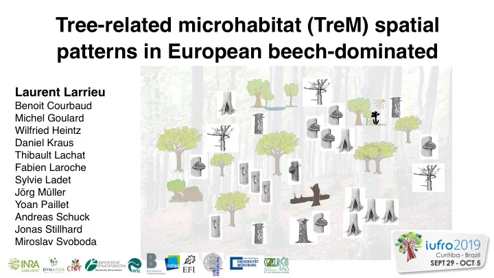
Tree-related microhabitat (TreM) spatial patterns in European beech-dominated forests Laurent Larrieu Benoit Courbaud Michel Goulard Wilfried Heintz Daniel Kraus Thibault Lachat Fabien Laroche Sylvie Ladet Jörg Müller Yoan Paillet Andreas Schuck Jonas Stillhard Miroslav Svoboda

Introductio M&M Results: Plot scale/Set of plots scale/Forest massif scale/TreM/Set of TreMs Conclusion n Are spatial distribution patterns of TreMs different in harvested stands compared to unharvested ones? Hypothesis 1: TreM distribution is spatially structured in old-growth forests (>100 years) Hypothesis 2: The spatial distribution of TreMs is mainly driven by the spatial distribution of tree dbh Hypothesis 3: Management affects these patterns by controlling dbh range, density and location of TreM-bearing trees

Introduction M&M Results: Plot scale/Set of plots scale/Forest massif scale/TreM/Set of TreMs Conclusion Unharvested forest A multi-scale explanatory analysis Harvested and unharvested stands r N Forest scale (Uholka, OGF) • • Set of 6 TreMs pooled 8 individual TreMs • • Marked point process (MPP) Binomial GLM/GLMM 408 plots • 266 x 500m ² -plots N, mean dbh N, mean dbh d d Plot-grouping scale Plot • Set of 6 TreMs pooled scale • Set of 6 TreMs pooled • Binomial GLM • 11 individual TreMs • Y (tree bears at least a • Binomial GLM TreM)~dbh+site+site-plot +time since the • Y (tree bears at least a TreM)~dbh+ 6 last harvest TreM-bearing tree variables describing neighbourhood

Outils statistiques et informatiques ● Library spat-stats : processus ponctuels marqués ● Marques : présence d’un ou de plusieurs TREMS ● Fonction L(r) : -> E{ arbres porteurs (non-porteurs) à moins de r d’un arbre observé porteurs (ou non porteurs)} , enveloppe sous hypothèse permutation des marques ● Utilisation des fonctions sous-jacentes pour calculer des valeurs individuelles : distance au plus proches voisins marqué ou non, nombre de points marqués (ou non marqués dans un voisinage)

Introduction M&M Results : Plot scale /Set of plots scale/Forest massif scale/TreM/ Set of TreMs Conclusion No consistent spatial pattern, neither in managed nor in old growth forests r General case MPP without control of the spatial Aggregation structure for dbh of marked trees But very rarely… L 1,1 (r) Repulsion random distribution of the TreM-bearing trees Confidence interval L1,1 (r) function: counts the nb of TreM-bearing trees in the r-radius disc

Introduction Spatial patterns Spatial patterns Old growth forests Old growth forests Managed stands TreM-dwelling taxa Practical issues Time since the last harvest influences the spatial pattern of the TreM-bearing trees Significant deviation values Deviance explained by the model compared to null model Fagus sylvatica 50% > • 25 sites/165 plots/11425 trees • 11 TreM groups • GLM binomial (Y=with a TreM or not) • 4 variables describing tree- neighborhood -d to the closer TreM-bearing tree -d to the closer tree without TreM -nb TreM-bearing trees in a 40m- >100y 50-100y <50y buffer Time since the last harvest -nb trees without TreM in a 40m-

Introduction M&M Results : Plot scale /Set of plots scale/Forest massif scale/TreM/ Set of TreMs Conclusion Neighbourhood features have a significant d effect on TreM bearing tree occurrence d GLM binomial Y=tree bears a TreM or not for 25% of the plots in Old-growth forest for 50 % of the plots in Managed forest + 10% of variance explained by neighbourhood + 18% of variance explained by neighbourhood (in addition to dbh) (in addition to dbh)

Introduction M&M Results : Plot scale / Set of plots scale / Forest massif scale / TreM / Set of TreMs Conclusion The effect of dbh on TreM occurrence depends on both TreM and forest status GLM binomial Y=tree bears a TreM or not Managed forest TreM Old Growth Forests Dbh effect + + for 88% of the plots + for 52% of the plots + - + + for 94% of the plots - for 65% of the plots + for 100% of the plots + for 97% of the plots = % var. explained by plot:dbh >> % var. explained by dbh

Introduction M&M Results : Plot scale / Set of plots scale / Forest massif scale / TreM / Set of TreMs Conclusion Local conditions are the main driver of TreM occurrence GLM binomial Y=tree bears a TreM or not ➢ dbh ***, but low explanatory power (3%) ➢ Time since the last harvest (dbh*time) ***, medium explanatory power (17%) ➢ Site (dbh*site)***, high explanatory power (36%) ➢ Site-plot (dbh*site-plot)***, the highest explanatory power (42%) Same trend observed at the individually TreM level!

Introduction M&M Results : Plot scale / Set of plots scale / Forest massif scale / TreM / Set of TreMs Conclusion Plot features and especially canopy cover matters for explaining the occurrence of most of the TreMs Drivers TreMs GLM & GLMM, binomial Y=tree bears a TreM or not + + ➢ DBH - - - ➢ Plot features • canopy cover + • slope + + • elevation