Tractable Representations Inference Probabilistic Learning - PowerPoint PPT Presentation
Tractable Representations Inference Probabilistic Learning Models Applications Guy Van den Broeck University of California, Los Angeles based on a joint UAI-19 tutorial with Antonio Vergari University of California, Los Angeles Nicola Di
Variational Autoencoders ∫ p θ ( x ) = p θ ( x | z ) p ( z ) d z an explicit likelihood model! Rezende et al., “Stochastic backprop. and approximate inference in deep generative models”, 2014 16 /89 Kingma et al., “Auto-Encoding Variational Bayes”, 2014
Variational Autoencoders [ ] log p θ ( x ) ≥ E z ∼ q ϕ ( z | x ) log p θ ( x | z ) − KL ( q φ ( z | x ) || p ( z )) an explicit likelihood model! ... but computing log p θ ( x ) is intractable an infinite and uncountable mixture ⇒ ⇒ no tractable EVI we need to optimize the ELBO… which is “broken” ⇒ [Alemi et al. 2017; Dai et al. 2019] 17 /89
Probabilistic Graphical Models (PGMs) Declarative semantics : a clean separation of modeling assumptions from inference Nodes : random variables X 1 X 3 Edges : dependencies X 5 + X 2 X 4 Inference : conditioning [Darwiche 2001; Sang et al. 2005] elimination [Zhang et al. 1994; Dechter 1998] message passing [Yedidia et al. 2001; Dechter et al. 2002; Choi et al. 2010; Sontag et al. 2011] 18 /89
PGMs: MNs and BNs Markov Networks (MNs) X 1 X 3 p ( X ) = 1 ∏ c φ c ( X c ) Z X 5 X 2 X 4 19 /89
PGMs: MNs and BNs Markov Networks (MNs) X 1 X 3 p ( X ) = 1 ∏ c φ c ( X c ) Z X 5 ∫ ∏ Z = c φ c ( X c ) d X X 2 X 4 ⇒ EVI queries are intractable! 19 /89
PGMs: MNs and BNs Markov Networks (MNs) X 1 X 3 p ( X ) = 1 ∏ c φ c ( X c ) Z X 5 ∫ ∏ Z = c φ c ( X c ) d X X 2 X 4 ⇒ EVI queries are intractable! Bayesian Networks (BNs) X 1 X 3 p ( X ) = ∏ i p ( X i | pa ( X i )) X 5 X 2 EVI queries are tractable! ⇒ X 4 19 /89
pinterest.com/pin/190417890473268205/ Marginal queries (MAR) q 1 : What is the probability that today is a Monday at 12.00 and there is a traffic jam only on Herzl Str.? 20 /89
pinterest.com/pin/190417890473268205/ Marginal queries (MAR) q 1 : What is the probability that today is a Monday at 12.00 and there is a traffic jam only on Herzl Str.? q 1 ( m ) = p m ( Day = Mon , Jam Herzl = 1) 20 /89
pinterest.com/pin/190417890473268205/ Marginal queries (MAR) q 1 : What is the probability that today is a Monday at 12.00 and there is a traffic jam only on Herzl Str.? q 1 ( m ) = p m ( Day = Mon , Jam Herzl = 1) General: p m ( e ) = ∫ p m ( e , H ) d H where E ⊂ X H = X \ E 20 /89
pinterest.com/pin/190417890473268205/ Conditional queries (CON) q 4 : What is the probability that there is a traffic jam on Herzl Str. given that today is a Monday? 21 /89
pinterest.com/pin/190417890473268205/ Conditional queries (CON) q 4 : What is the probability that there is a traffic jam on Herzl Str. given that today is a Monday? q 4 ( m ) = p m ( Jam Herzl = 1 | Day = Mon ) 21 /89
pinterest.com/pin/190417890473268205/ Conditional queries (CON) q 4 : What is the probability that there is a traffic jam on Herzl Str. given that today is a Monday? q 4 ( m ) = p m ( Jam Herzl = 1 | Day = Mon ) If you can answer MAR queries, then you can also do conditional queries ( CON ): p m ( Q | E ) = p m ( Q , E ) p m ( E ) 21 /89
Complexity of MAR on PGMs Exact complexity: Computing MAR and COND is #P-complete [Cooper 1990; Roth 1996]. Approximation complexity: Computing MAR and COND approximately within a relative error of 2 n 1 − ϵ for any fixed ϵ is NP-hard [Dagum et al. 1993; Roth 1996]. Treewidth : Informally, how tree-like is the graphical model m ? Formally, the minimum width of any tree-decomposition of m . Fixed-parameter tractable : MAR and CON on a graphical model m with treewidth w take time O ( | X | · 2 w ) , which is linear for fixed width w [Dechter 1998; Koller et al. 2009]. what about bounding the treewidth by design? ⇒ 22 /89
Complexity of MAR on PGMs Exact complexity: Computing MAR and COND is #P-complete [Cooper 1990; Roth 1996]. Approximation complexity: Computing MAR and COND approximately within a relative error of 2 n 1 − ϵ for any fixed ϵ is NP-hard [Dagum et al. 1993; Roth 1996]. Treewidth : Informally, how tree-like is the graphical model m ? Formally, the minimum width of any tree-decomposition of m . Fixed-parameter tractable : MAR and CON on a graphical model m with treewidth w take time O ( | X | · 2 w ) , which is linear for fixed width w [Dechter 1998; Koller et al. 2009]. what about bounding the treewidth by design? ⇒ 22 /89
Low-treewidth PGMs X 1 X 1 X 3 X 3 X 1 X 2 X 3 X 5 X 2 X 5 X 2 X 5 X 1 X 3 X 4 X 4 X 4 Trees Polytrees Thin Junction trees [Meilă et al. 2000] [Dasgupta 1999] [Bach et al. 2001] If treewidth is bounded (e.g. ≊ 20 ), exact MAR and CON inference is possible in practice 23 /89
Low-treewidth PGMs: trees A tree-structured BN [Meilă et al. 2000] where each X i ∈ X has at most one parent Pa X i . X 1 X 3 ∏ n p ( X ) = i =1 p ( x i | Pa x i ) X 5 X 2 X 4 Exact querying: EVI, MAR, CON tasks linear for trees : O ( | X | ) Exact learning from d examples takes O ( | X | 2 · d ) with the classical Chow-Liu algorithm 1 24 /89 1 Chow et al., “Approximating discrete probability distributions with dependence trees”, 1968
What do we lose? Expressiveness : Ability to compactly represent rich and complex classes of distributions X 1 X 3 X 5 X 2 X 4 Bounded-treewidth PGMs lose the ability to represent all possible distributions … Cohen et al., “On the expressive power of deep learning: A tensor analysis”, 2016 25 /89 Martens et al., “On the Expressive Efficiency of Sum Product Networks”, 2014
Mixtures Mixtures as a convex combination of k (simpler) probabilistic models 0 . 25 0 . 20 p ( X 1 ) 0 . 15 p ( X ) = w 1 · p 1 ( X )+ w 2 · p 2 ( X ) 0 . 10 0 . 05 0 . 00 − 10 − 5 0 5 10 X 1 EVI, MAR, CON queries scale linearly in k 26 /89
Mixtures Mixtures as a convex combination of k (simpler) probabilistic models 0 . 25 p ( X ) = p ( Z = 1 ) · p 1 ( X | Z = 1 ) 0 . 20 p ( X 1 ) + p ( Z = 2 ) · p 2 ( X | Z = 2 ) 0 . 15 0 . 10 0 . 05 0 . 00 − 10 − 5 0 5 10 X 1 Mixtures are marginalizing a categorical latent variable Z with k values ⇒ increased expressiveness 26 /89
Expressiveness and efficiency Expressiveness : Ability to compactly represent rich and effective classes of functions mixture of Gaussians can approximate any distribution! ⇒ Expressive efficiency (succinctness) compares model sizes in terms of their ability to compactly represent functions but how many components do they need? ⇒ Cohen et al., “On the expressive power of deep learning: A tensor analysis”, 2016 27 /89 Martens et al., “On the Expressive Efficiency of Sum Product Networks”, 2014
Mixture models Expressive efficiency deeper mixtures would be efficient compared to shallow ones ⇒ 28 /89
pinterest.com/pin/190417890473268205/ Maximum A Posteriori (MAP) aka Most Probable Explanation (MPE) q 5 : Which combination of roads is most likely to be jammed on Monday at 9am? 29 /89
pinterest.com/pin/190417890473268205/ Maximum A Posteriori (MAP) aka Most Probable Explanation (MPE) q 5 : Which combination of roads is most likely to be jammed on Monday at 9am? q 5 ( m ) = argmax j p m ( j 1 , j 2 , . . . | Day = M , Time = 9 ) 29 /89
pinterest.com/pin/190417890473268205/ Maximum A Posteriori (MAP) aka Most Probable Explanation (MPE) q 5 : Which combination of roads is most likely to be jammed on Monday at 9am? q 5 ( m ) = argmax j p m ( j 1 , j 2 , . . . | Day = M , Time = 9 ) General: argmax q p m ( q | e ) where Q ∪ E = X 29 /89
pinterest.com/pin/190417890473268205/ Maximum A Posteriori (MAP) aka Most Probable Explanation (MPE) q 5 : Which combination of roads is most likely to be jammed on Monday at 9am? …intractable for latent variable models! ∑ max p m ( q | e ) = max p m ( q , z | e ) q q z ∑ ̸ = max p m ( q , z | e ) q z 29 /89
pinterest.com/pin/190417890473268205/ Marginal MAP (MMAP) aka Bayesian Network MAP q 6 : Which combination of roads is most likely to be jammed on Monday at 9am? 30 /89
pinterest.com/pin/190417890473268205/ Marginal MAP (MMAP) aka Bayesian Network MAP q 6 : Which combination of roads is most likely to be jammed on Monday at 9am? q 6 ( m ) = argmax j p m ( j 1 , j 2 , . . . | Time = 9 ) 30 /89
pinterest.com/pin/190417890473268205/ Marginal MAP (MMAP) aka Bayesian Network MAP q 6 : Which combination of roads is most likely to be jammed on Monday at 9am? q 6 ( m ) = argmax j p m ( j 1 , j 2 , . . . | Time = 9 ) General: argmax q p m ( q | e ) ∑ = argmax q h p m ( q , h | e ) where Q ∪ H ∪ E = X 30 /89
pinterest.com/pin/190417890473268205/ Marginal MAP (MMAP) aka Bayesian Network MAP q 6 : Which combination of roads is most likely to be jammed on Monday at 9am? q 6 ( m ) = argmax j p m ( j 1 , j 2 , . . . | Time = 9 ) NP PP -complete [Park et al. 2006] ⇒ NP-hard for trees [Campos 2011] ⇒ ⇒ NP-hard even for Naive Bayes [ibid.] 30 /89
pinterest.com/pin/190417890473268205/ Advanced queries q 2 : Which day is most likely to have a traffic jam on my route to work? 31 /89 Bekker et al., “Tractable Learning for Complex Probability Queries”, 2015
pinterest.com/pin/190417890473268205/ Advanced queries q 2 : Which day is most likely to have a traffic jam on my route to work? q 2 ( m ) = argmax d p m ( Day = d ∧ ∨ i ∈ route Jam Str i ) marginals + MAP + logical events ⇒ 31 /89 Bekker et al., “Tractable Learning for Complex Probability Queries”, 2015
pinterest.com/pin/190417890473268205/ Advanced queries q 2 : Which day is most likely to have a traffic jam on my route to work? q 7 : What is the probability of seeing more traffic jams in Jaffa than Marina? 31 /89 Bekker et al., “Tractable Learning for Complex Probability Queries”, 2015
pinterest.com/pin/190417890473268205/ Advanced queries q 2 : Which day is most likely to have a traffic jam on my route to work? q 7 : What is the probability of seeing more traffic jams in Jaffa than Marina? counts + group comparison ⇒ 31 /89 Bekker et al., “Tractable Learning for Complex Probability Queries”, 2015
pinterest.com/pin/190417890473268205/ Advanced queries q 2 : Which day is most likely to have a traffic jam on my route to work? q 7 : What is the probability of seeing more traffic jams in Jaffa than Marina? and more: expected classification agreement [Oztok et al. 2016; Choi et al. 2017, 2018] expected predictions [Khosravi et al. 2019a] 31 /89 Bekker et al., “Tractable Learning for Complex Probability Queries”, 2015
Fully factorized models A completely disconnected graph. Example: Product of Bernoullis (PoBs) X 1 ∏ n p ( X ) = i =1 p ( x i ) X 3 X 5 X 2 X 4 Complete evidence, marginals and MAP, MMAP inference is linear ! ⇒ but definitely not expressive… 32 /89
more tractable queries more expressive less expressive efficient efficient less tractable queries 33 /89
more tractable queries more expressive less expressive efficient efficient NADEs BNs NFs MNs VAEs GANs less tractable queries Expressive models are not very tractable… 34 /89
more tractable queries Fully factorized LTM Trees NB Mixtures Polytrees TJT more expressive less expressive efficient efficient NADEs BNs NFs MNs VAEs GANs less tractable queries and tractable ones are not very expressive… 35 /89
more tractable queries X Fully factorized LTM Trees NB Mixtures Polytrees TJT more expressive less expressive efficient efficient NADEs BNs NFs MNs VAEs GANs less tractable queries probabilistic circuits are at the “sweet spot” 36 /89
Probabilistic Circuits
Stay Tuned For … Next: 1. What are the building blocks of tractable models? a computational graph forming a probabilistic circuit ⇒ 2. For which queries are probabilistic circuits tractable? tractable classes induced by structural properties ⇒ After: How are probabilistic circuits related to the alphabet soup of models? 38 /89
Base Case: Univariate Distributions p X ( x ) x X Generally, univariate distributions are tractable for: EVI : output p ( X i ) (density or mass) MAR : output 1 (normalized) or Z (unnormalized) MAP : output the mode 39 /89
Base Case: Univariate Distributions p X ( x ) x X Generally, univariate distributions are tractable for: EVI : output p ( X i ) (density or mass) MAR : output 1 (normalized) or Z (unnormalized) MAP : output the mode ⇒ often 100% probability for one value of a categorical random variable for example, X or ¬ X for Boolean random variable ⇒ 39 /89
Base Case: Univariate Distributions . 74 . 33 X Generally, univariate distributions are tractable for: EVI : output p ( X i ) (density or mass) MAR : output 1 (normalized) or Z (unnormalized) MAP : output the mode ⇒ often 100% probability for one value of a categorical random variable for example, X or ¬ X for Boolean random variable ⇒ 39 /89
Factorizations are products Divide and conquer complexity p ( X 1 , X 2 , X 3 ) = p ( X 1 ) · p ( X 2 ) · p ( X 3 ) 3 . 0 X 1 × 2 . 5 2 . 0 X 2 1 . 5 1 . 0 X 3 0 . 5 X 1 X 2 X 3 0 . 0 X 1 X 2 X 3 e.g. modeling a multivariate Gaussian with diagonal covariance matrix ⇒ 40 /89
Factorizations are products Divide and conquer complexity p ( x 1 , x 2 , x 3 ) = p ( x 1 ) · p ( x 2 ) · p ( x 3 ) 3 . 0 X 1 × 2 . 5 2 . 0 X 2 1 . 5 0.8 0.5 0.9 1 . 0 X 3 0 . 5 X 1 X 2 X 3 0 . 0 X 1 X 2 X 3 e.g. modeling a multivariate Gaussian with diagonal covariance matrix ⇒ 40 /89
Factorizations are products Divide and conquer complexity p ( x 1 , x 2 , x 3 ) = p ( x 1 ) · p ( x 2 ) · p ( x 3 ) 3 . 0 X 1 .36 2 . 5 2 . 0 X 2 1 . 5 0.5 0.8 0.9 1 . 0 X 3 0 . 5 X 1 X 2 X 3 0 . 0 X 1 X 2 X 3 e.g. modeling a multivariate Gaussian with diagonal covariance matrix ⇒ 40 /89
Mixtures are sums Also mixture models can be treated as a simple computational unit over distributions 0 . 25 0 . 20 p ( X 1 ) 0 . 15 p ( X ) = w 1 · p 1 ( X )+ w 2 · p 2 ( X ) 0 . 10 0 . 05 0 . 00 − 10 − 5 0 5 10 X 1 41 /89
Mixtures are sums Also mixture models can be treated as a simple computational unit over distributions w 1 w 2 p ( x ) = 0 . 2 · p 1 ( x )+0 . 8 · p 2 ( x ) X 1 X 1 41 /89
Mixtures are sums Also mixture models can be treated as a simple computational unit over distributions .44 0 . 2 0 . 8 p ( x ) = 0 . 2 · p 1 ( x )+0 . 8 · p 2 ( x ) 0.2 0.5 X 1 X 1 With mixtures, we increase expressiveness ⇒ by stacking them we increase expressive efficiency 41 /89
A grammar for tractable models Recursive semantics of probabilistic circuits X 1 42 /89
A grammar for tractable models Recursive semantics of probabilistic circuits w 1 w 2 X 1 X 1 X 1 42 /89
A grammar for tractable models Recursive semantics of probabilistic circuits w 1 w 2 × × w 1 w 2 X 1 X 1 X 1 X 1 X 2 X 1 X 2 42 /89
A grammar for tractable models Recursive semantics of probabilistic circuits X 1 X 1 × × w 1 w 2 X 2 X 2 × × w 1 w 2 × × × × X 1 X 1 X 1 X 3 X 4 X 3 X 4 X 1 X 2 X 1 X 2 42 /89
Probabilistic circuits are not PGMs! They are probabilistic and graphical , however … PGMs Circuits Nodes : random variables unit of computations Edges : dependencies order of execution Inference : conditioning feedforward pass elimination backward pass message passing ⇒ they are computational graphs, more like neural networks 43 /89
Just sum, products and distributions? X 1 × × X 2 × × × X 3 × × × X 4 × × × X 5 × × × X 6 × × just arbitrarily compose them like a neural network! 44 /89
Just sum, products and distributions? X 1 × × X 2 × × × X 3 × × × X 4 × × × X 5 × × × X 6 × × just arbitrarily compose them like a neural network! structural constraints needed for tractability ⇒ 44 /89
How do we ensure tractability? 45 /89
Decomposability A product node is decomposable if its children depend on disjoint sets of variables just like in factorization! ⇒ × × X 1 X 2 X 3 X 1 X 1 X 3 decomposable circuit non-decomposable circuit 46 /89 Darwiche et al., “A knowledge compilation map”, 2002
Smoothness aka completeness A sum node is smooth if its children depend of the same variable sets otherwise not accounting for some variables ⇒ w 1 w 2 w 1 w 2 X 1 X 1 X 1 X 2 smooth circuit non-smooth circuit smoothness can be easily enforced [Shih et al. 2019] ⇒ 47 /89 Darwiche et al., “A knowledge compilation map”, 2002
Tractable MAR/CON Smoothness and decomposability enable tractable MAR/CON queries X 1 X 1 × × X 2 X 2 × × × × X 3 X 4 X 3 X 4 48 /89
Tractable MAR/CON Smoothness and decomposability enable tractable MAR/CON queries If p ( x , y ) = p ( x ) p ( y ) , ( decomposability ): X 1 X 1 × × ∫ ∫ ∫ ∫ X 2 X 2 p ( x , y ) d x d y = p ( x ) p ( y ) d x d y = ∫ ∫ × × × × = p ( x ) d x p ( y ) d y X 3 X 4 X 3 X 4 larger integrals decompose into easier ones ⇒ 48 /89
Tractable MAR/CON Smoothness and decomposability enable tractable MAR/CON queries If p ( x ) = ∑ i w i p i ( x ) , ( smoothness ): X 1 X 1 × × ∫ ∫ ∑ X 2 X 2 p ( x ) d x = w i p i ( x ) d x = i × × × × ∫ ∑ = p i ( x ) d x w i i X 3 X 4 X 3 X 4 ⇒ integrals are “pushed down” to children 48 /89
Tractable MAR/CON Smoothness and decomposability enable tractable MAR/CON queries .49 Forward pass evaluation for MAR linear in circuit size! ⇒ 1.0 .35 .64 1.0 E.g. to compute p ( x 2 , x 4 ) : .61 .58 .77 .83 leafs over X 1 and X 3 output Z i = ∫ p ( x i ) dx i .58 .58 .77 .77 ⇒ for normalized leaf distributions: 1 . 0 leafs over X 2 and X 4 output EVI 1.0 .58 1.0 .77 48 /89
Determinism aka selectivity A sum node is deterministic if the output of only one children is non zero for any input e.g. if their distributions have disjoint support ⇒ w 1 w 2 w 1 w 2 × × × × X 1 ≤ θ X 2 X 1 > θ X 2 X 1 X 2 X 1 X 2 deterministic circuit non-deterministic circuit 49 /89
Tractable MAP The addition of determinism enables tractable MAP queries! X 1 X 1 × × X 2 X 2 × × × × X 3 X 4 X 3 X 4 50 /89
Tractable MAP The addition of determinism enables tractable MAP queries! If p ( q , e ) = p ( q x , e x , q y , e y ) = p ( q x , e x ) p ( q y , e y ) ( decomposable product node): X 1 X 1 × × argmax p ( q | e ) = argmax p ( q , e ) q q X 2 X 2 = argmax p ( q x , e x , q y , e y ) q x , q y × × × × = argmax p ( q x , e x ) , argmax p ( q y , e y ) q x q y X 3 X 4 X 3 X 4 solving optimization independently ⇒ 50 /89
Tractable MAP The addition of determinism enables tractable MAP queries! If p ( q , e ) = ∑ i w i p i ( q , e ) = w c p c ( q , e ) , ( deterministic sum node): X 1 X 1 × × ∑ argmax p ( q , e ) = argmax w i p i ( q , e ) q q i X 2 X 2 = argmax max w i p i ( q , e ) i q × × × × = max argmax w i p i ( q , e ) i q X 3 X 4 X 3 X 4 one non-zero child term, thus sum is max ⇒ 50 /89
Tractable MAP The addition of determinism enables tractable MAP queries! Evaluating the circuit twice: bottom-up and top-down still linear in circuit size! ⇒ X 1 X 1 × × X 2 X 2 × × × × X 3 X 4 X 3 X 4 50 /89
Tractable MAP The addition of determinism enables tractable MAP queries! Evaluating the circuit twice: max bottom-up and top-down still linear in circuit size! ⇒ X 1 X 1 × × In practice: X 2 X 2 max max 1. turn sum into max nodes 2. evaluate p ( e ) bottom-up × × × × 3. retrieve max activations top-down 4. compute MAP queries at leaves X 3 X 4 X 3 X 4 50 /89
Tractable MAP The addition of determinism enables tractable MAP queries! Evaluating the circuit twice: max bottom-up and top-down still linear in circuit size! ⇒ X 1 X 1 × × In practice: X 2 X 2 max max 1. turn sum into max nodes 2. evaluate p ( e ) bottom-up × × × × 3. retrieve max activations top-down 4. compute MAP queries at leaves X 3 X 4 X 3 X 4 50 /89
Recommend
More recommend
Explore More Topics
Stay informed with curated content and fresh updates.
