Towards a More Realistic Proof of the Main Result Treatment of - PowerPoint PPT Presentation

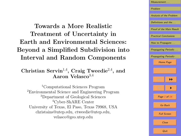
Measurement . . . Problem Analysis of the Problem Definitions and the . . . Towards a More Realistic Proof of the Main Result Treatment of Uncertainty in Practical Conclusions Earth and Environmental Sciences: How to Propagate . . . Beyond a Simplified Subdivision into Propagating Periodic . . . Interval and Random Components Propagating Periodic- . . . Home Page Christian Servin 1 , 4 , Craig Tweedie 2 , 4 , and Title Page Aaron Velasco 3 , 4 ◭◭ ◮◮ 1 Computational Sciences Program ◭ ◮ 2 Environmental Science and Engineering Program 3 Department of Geological Sciences Page 1 of 14 4 Cyber-ShARE Center Go Back University of Texas, El Paso, Texas 79968, USA christains@utep.edu, ctweedie@utep.edu, Full Screen velasco@geo.utep.edu Close Quit

Measurement . . . Problem 1. Measurement Uncertainty: Reminder Analysis of the Problem def • Usually, a meas. error ∆ x = � x − x is subdivided into Definitions and the . . . random and systematic components ∆ x = ∆ s x + ∆ r x : Proof of the Main Result Practical Conclusions – the systematic error component ∆ s x is usually de- How to Propagate . . . fined as the expected value ∆ s x = E [∆ x ], while Propagating Periodic . . . – the random error component is usually defined as Propagating Periodic- . . . def the difference ∆ r x = ∆ x − ∆ s x . Home Page • The random errors ∆ r x corresponding to different mea- Title Page surements are usually assumed to be independent. ◭◭ ◮◮ • For ∆ s x , we only know the upper bound ∆ s s.t. ◭ ◮ | ∆ s x | ≤ ∆ s , i.e., that ∆ s x is in the interval [ − ∆ s , ∆ s ]. Page 2 of 14 • Because of this fact, interval computations are used for processing the systematic errors. Go Back Full Screen • ∆ r x is usually characterized by the corr. probability distribution (usually Gaussian, with known σ ). Close Quit

Measurement . . . Problem 2. Problem Analysis of the Problem • Often, the differences ∆ r x = ∆ x − ∆ s x corr. to nearby Definitions and the . . . times are strongly correlated. Proof of the Main Result Practical Conclusions • For example, meteorological sensors may have daytime How to Propagate . . . or nighttime biases, or winter and summer biases. Propagating Periodic . . . • To capture this correlation, environmental scientists Propagating Periodic- . . . proposed a semi-heuristic 3-component model of ∆ x . Home Page • In this model, the difference ∆ x − ∆ s x is represented Title Page as a combination of: ◭◭ ◮◮ – a “truly random” error ∆ t x (which is independent ◭ ◮ from one measurement to another), and Page 3 of 14 – a new “periodic” component ∆ p x . Go Back • We provide a theoretical explanation for this heuristic Full Screen three-component model. Close Quit

Measurement . . . Problem 3. Analysis of the Problem Analysis of the Problem • We want to represent measurement error ∆ x ( t ) as a Definitions and the . . . linear combination of several components. Proof of the Main Result Practical Conclusions • We consider the most detailed level of granularity, w/each How to Propagate . . . component determined by finitely many parameters c i . Propagating Periodic . . . • Each component is thus described by a finite-dimensional Propagating Periodic- . . . linear space Home Page L = { c 1 · x 1 ( t ) + . . . + c n · x n ( t ) : c 1 , . . . , c n ∈ I R } . Title Page • In most applications, signals are smooth and bounded, ◭◭ ◮◮ so we assume that x i ( t ) is smooth and bounded. ◭ ◮ • Finally, for a long series of observations, we can choose Page 4 of 14 a starting point arbitrarily: t → t + t 0 . Go Back • It is reasonable to require that this change keeps us Full Screen within the same component, i.e., Close x ( t ) ∈ L ⇒ x ( t + t 0 ) ∈ L. Quit

Measurement . . . Problem 4. Definitions and the Main Result Analysis of the Problem • A function x ( t ) of one variable is called bounded if Definitions and the . . . Proof of the Main Result ∃ M ∀ t ( | x ( t ) | ≤ M ) . Practical Conclusions How to Propagate . . . • We say that a class F of functions of one variable is shift-invariant if Propagating Periodic . . . Propagating Periodic- . . . ∀ x ( t ) ( x ( t ) ∈ F ⇒ ∀ t 0 ( x ( t + t 0 ) ∈ F )) . Home Page Title Page • By an error component we mean a shift-invariant finite- dimensional linear space of functions ◭◭ ◮◮ L = { c 1 · x 1 ( t ) + . . . + c n · x n ( t ) : c i ∈ I R } . ◭ ◮ Page 5 of 14 • Theorem: Every error component is a linear combi- Go Back nation of the functions Full Screen x ( t ) = sin( ω · t ) and x ( t ) = cos( ω · t ) . Close Quit

Measurement . . . Problem 5. Proof of the Main Result Analysis of the Problem • Shift-invariance means that, for some c i ( t 0 ), we have Definitions and the . . . Proof of the Main Result x i ( t + t 0 ) = c i 1 ( t 0 ) · x 1 ( t ) + . . . + c in ( t 0 ) · x n ( t ) . Practical Conclusions How to Propagate . . . • For n different values t = t 1 , . . . , t = t n , we get a system of n linear equations with n unknowns c ij ( t 0 ). Propagating Periodic . . . Propagating Periodic- . . . • The Cramer’s rule solution to linear equations is a Home Page smooth function of all the coeff. & right-hand sides. Title Page • Since all the right-hand sides x i ( t j + t 0 ) and coefficients ◭◭ ◮◮ x i ( t j ) are smooth, c ij ( t 0 ) are also smooth. ◭ ◮ def • Differentiating w.r.t. t 0 and taking t 0 = 0, for c ij = Page 6 of 14 c ij (0), we get ˙ Go Back x i ( t ) = c i 1 · x 1 ( t ) + . . . + c in · x n ( t ) . ˙ Full Screen Close Quit

Measurement . . . Problem 6. Proof (cont-d) Analysis of the Problem • Reminder: ˙ x i ( t ) = c i 1 · x 1 ( t ) + . . . + c in · x n ( t ) . Definitions and the . . . Proof of the Main Result • A general solution of such system of equations is a lin- Practical Conclusions ear combination of functions How to Propagate . . . t k · exp( λ · t ) , w/ k ∈ N , k ≥ 0 , λ = a + i · ω ∈ C . Propagating Periodic . . . Propagating Periodic- . . . • Here, Home Page exp( λ · t ) = exp( a · t ) · cos( ω · t ) + i · exp( a · t ) · sin( ω · t ) . Title Page ◭◭ ◮◮ • When a � = 0, we get unbounded functions for t → ∞ or t → −∞ . ◭ ◮ • So, a = 0. Page 7 of 14 • For k > 0, we get unbounded t k ; so, k = 0. Go Back Full Screen • Thus, we indeed have a linear combination of sinusoids. Close Quit

Measurement . . . Problem 7. Practical Conclusions Analysis of the Problem • Let f be the measurements frequency (how many mea- Definitions and the . . . surements we perform per unit time). Proof of the Main Result Practical Conclusions • When ω ≪ f , the values cos( ω · t ) and sin( ω · t ) prac- How to Propagate . . . tically do not change with time. Propagating Periodic . . . • Indeed, the change period is much larger than the usual Propagating Periodic- . . . observation period. Home Page • Thus, we can identify such low-frequency components Title Page with systematic error component. ◭◭ ◮◮ • When ω ≫ f , the phases of the values cos( ω · t i ) and ◭ ◮ cos( ω · t i +1 ) differ a lot. Page 8 of 14 • For all practical purposes, the resulting values of cosine or sine functions are independent. Go Back Full Screen • Thus, high-frequency components can be identified with random error component. Close Quit

Measurement . . . Problem 8. Practical Conclusions (cont-d) Analysis of the Problem • Result: every error component is a linear combination Definitions and the . . . of cos( ω · t ) and sin( ω · t ) . Proof of the Main Result Practical Conclusions • Notation: let f be the measurements frequency (how How to Propagate . . . many measurements we perform per unit time). Propagating Periodic . . . • Reminder: Propagating Periodic- . . . Home Page – we can identify low-frequency components ( ω ≪ f ) with systematic error component; Title Page – we can identify high-frequency ones ( ω ≫ f ) with ◭◭ ◮◮ random error component. ◭ ◮ • Easy to see: all other error components cos( ω · t ) and Page 9 of 14 sin( ω · t ) are periodic. Go Back • Conclusion: we have indeed justified to the semi-empirical Full Screen 3-component model of measurement error. Close Quit

Measurement . . . Problem 9. How to Propagate Uncertainty in the Three- Analysis of the Problem Component Model Definitions and the . . . • We are interested in the quantity Proof of the Main Result Practical Conclusions y = f ( x 1 ( t 11 ) , x 1 ( t 12 ) , . . . , x 2 ( t 21 ) , x 2 ( t 22 ) , . . . , x n ( t n 1 ) , x n ( t n 2 ) , . . . ) . How to Propagate . . . • Instead of the actual values x i ( t ij ), we only know the Propagating Periodic . . . measurement results � x i ( t ij ) = x i ( t ij ) + ∆ x i ( t ij ) . Propagating Periodic- . . . Home Page • Measurement errors are usually small, so terms quadratic (and higher) in ∆ x i ( t ij ) can be safely ignored. Title Page • For example, if the measurement error is 10%, its square ◭◭ ◮◮ is 1% which is much much smaller than 10%. ◭ ◮ • If the measurement error is 1%, its square is 0.01% Page 10 of 14 which is much much smaller than 1%. Go Back • Thus, we can safely linearize the dependence of ∆ y on Full Screen ∆ x i ( t ij ). Close Quit