Today Data Acquisition Systems Many embedded systems measure - PDF document

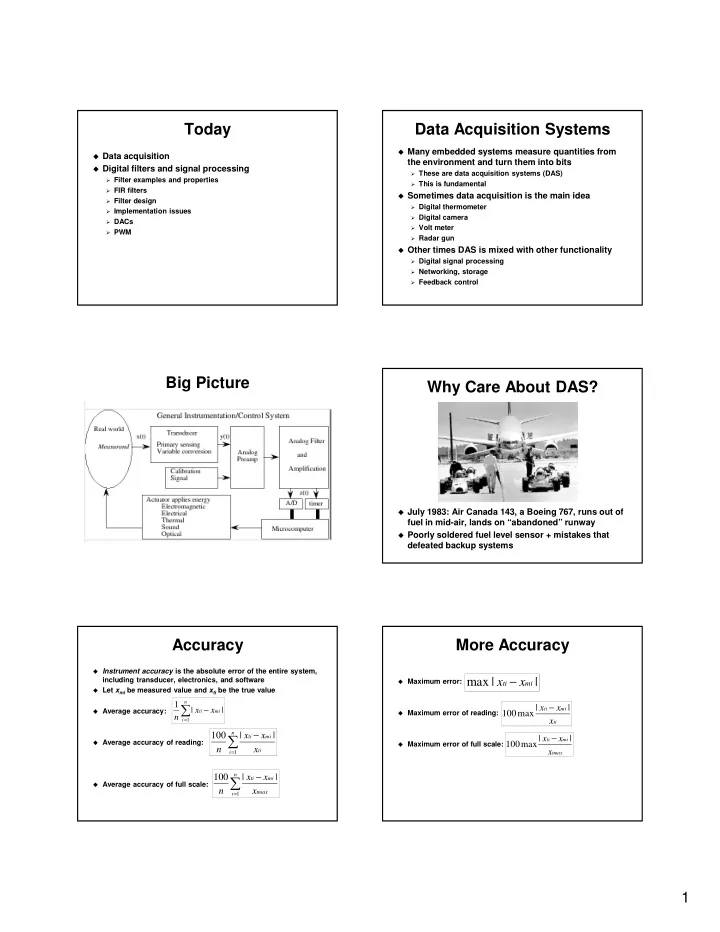
Today Data Acquisition Systems � Many embedded systems measure quantities from � Data acquisition the environment and turn them into bits � Digital filters and signal processing � These are data acquisition systems (DAS) � Filter examples and properties � This is fundamental � FIR filters � Sometimes data acquisition is the main idea � Filter design � Digital thermometer � Implementation issues � Digital camera � DACs � Volt meter � PWM � Radar gun � Other times DAS is mixed with other functionality � Digital signal processing � Networking, storage � Feedback control Big Picture Why Care About DAS? � July 1983: Air Canada 143, a Boeing 767, runs out of fuel in mid-air, lands on “abandoned” runway � Poorly soldered fuel level sensor + mistakes that defeated backup systems Accuracy More Accuracy � Instrument accuracy is the absolute error of the entire system, including transducer, electronics, and software max | x − x | � Maximum error: ti mi � Let x mi be measured value and x ti be the true value 1 n � | x x | | x x | ti − mi � Average accuracy: ti − mi � Maximum error of reading: 100 max n x i 1 = ti 100 n | | � x x ti − mi | x x | ti − mi � Average accuracy of reading: 100 max � Maximum error of full scale: n x ti x i 1 = tmax n 100 � | x x | ti − mi � Average accuracy of full scale: n x tmax 1 i = 1

Resolution Precision � Instrument resolution is the smallest input signal � Precision is number of distinguishable alternatives, difference that can be detected by the entire system n x , from which result is selected � May be limited by noise in either transducer or electronics � Can be expressed in bits or decimal digits � 1000 alternatives: 10 bits, 3 decimal digits � Spatial resolution of the transducer is the smallest � 2000 alternatives: 11 bits, 3.5 decimal digits distance between two independent measurements � 4000 alternatives: 12 bits, 3.75 decimal digits � 10000 alternatives: >13 bits, 4 decimal digits � Determined by size and mechanical properties of the � Range is resolution times precision: r x = � x n x transducer Reproducibility ADC: How many bits? � Reproducibility specifies whether the instrument has � Linear transducer case: equal outputs given identical inputs over some time � ADC resolution must be � problem resolution period � Nonlinear transducer case: � Specified as full range or standard deviation of � Let x be the real-world signal with range r x output results given a fixed input � Let y be the transducer output with range r y � Reproducibility errors often come from transducer � Let the required precision of x be n x � Resolutions of x and y are � x and � y drift � Transducer response described by y=f(x) � Required ADC precision n y (number of alternatives) is: • � x = r x /n x • � y = min { f(x + � x) – f(x) } for all x in r x � Bits is ceiling(log 2 n y ) ADC: How many bits? ADC: How many bits? smallest � y � x � x � ADC must be able to measure a change in voltage of � ADC must be able to measure a change in voltage of the smallest � y the smallest � y 2

DSP Big Picture Signal Reconstruction � Analog filter gets rid of unwanted high-frequency components in the output Data Acquisition Sampling � Signal: Time-varying measurable quantity whose � Transducers variation normally conveys information � Transducer turns a physical quantity into a voltage � Quantity often a voltage obtained from some transducer � ADC turns voltage into an n -bit integer � E.g. a microphone � Sampling is typically performed periodically � Sampling permits us to reconstruct signals from the world � Analog signals have infinitely variable values at all • E.g. sounds, seismic vibrations times � Key issue: aliasing � Digital signals are discrete in time and in value � Nyquist rate : 0.5 * sampling rate � Often obtained by sampling analog signals � Frequencies higher than the Nyquist rate get mapped to � Sampling produces sequence of numbers frequencies below the Nyquist rate • E.g. { ... , x[-2], x[-1], x[0], x[1], x[2], ... } � Aliasing cannot be undone by subsequent digital � These are time domain signals processing Sampling Theorem Aliasing Details � Discovered by Claude Shannon in 1949: � Let N be the sampling rate and F be a frequency found in the signal A signal can be reconstructed from its samples � Frequencies between 0 and 0.5*N are sampled properly without loss of information, if the original signal has � Frequencies >0.5*N are aliased no frequencies above 1/2 the sampling frequency • Frequencies between 0.5*N and N are mapped to (0.5*N)- F and have phase shifted 180 � � This is a pretty amazing result • Frequencies between N and 1.5*N are mapped to f-N with no phase shift � But note that it applies only to discrete time, not discrete values • Pattern repeats indefinitely � Aliasing may or may not occur when N == F*2*X where X is a positive integer 3

No Aliasing 1 kHz Signal, No Aliasing Aliasing Avoiding Aliasing Increase sampling rate 1. Not a general-purpose solution � White noise is not band-limited • • Faster sampling requires: – Faster ADC – Faster CPU – More power – More RAM for buffering Filter out undesirable frequencies before sampling 2. using analog filter(s) � This is what is done in practice � Analog filters are imperfect and require tradeoffs Signal Processing Pragmatics Aliasing in Space � Spatial sampling incurs aliasing problems also � Example: CCD in digital camera samples an image in a grid pattern � Real world is not band-limited � Can mitigate aliasing by increasing sampling rate Samples Pixel 4

Point vs. Supersampling Digital Signal Processing � Basic idea � Digital signals can be manipulated losslessly � SW control gives great flexibility � DSP examples � Amplification or attenuation � Filtering – leaving out some unwanted part of the signal � Rectification – making waveform purely positive � Modulation – multiplying signal by another signal • E.g. a high-frequency sine wave Point sampling 4x4 Supersampling Assumptions Filter Terms for CS People Signal sampled at fixed and known rate f s � Low pass – lets low frequency signals through, 1. suppresses high frequency I.e., ADC driven by timer interrupts � � High pass – lets high frequency signals through, Aliasing has not occurred suppresses low frequency 2. � I.e., signal has no significant frequency components � Passband – range of frequencies passed by a filter greater than 0.5*f s � Stopband – range of frequencies blocked These have to be removed before ADC using an analog � � Transition band – in between these filter Non-significant signals have amplitude smaller than the � ADC resolution Simple Digital Filters Gain vs. Frequency � y(n) = 0.5 * (x(n) + x(n-1)) 1.5 � Why not use x(n+1)? y(n) =(y(n-1)+x(n))/2 � y(n) = (1.0/6) * (x(n) + x(n-1) + x(n-2) + … + x(n-5) ) y(n) =(x(n)+x(n-1))/2 � y(n) = 0.5 * (x(n) + x(n-3)) y(n) =(x(n)+x(n-1)+x(n-2)+ 1.0 x(n-3)+x(n-4)+x(n-5))/6 � y(n) = 0.5 * (y(n-1) + x(n)) Gain � What makes this one different? y(n) =(x(n)+x(n-3))/2 � y(n) = median [ x(n) + x(n-1) + x(n-2) ] 0.5 0.0 0.0 0.1 0.2 0.3 0.4 0.5 frequency f/fs 5

Useful Signals Step Response 1 � Step: Step 1 0.8 � …, 0, 0, 0, 1, 1, 1, … s(n) step input Response 0.6 FIR 0.4 IIR -3 -2 -1 0 1 2 3 median 0.2 � Impulse: Impulse 1 i(n) � …, 0, 0, 0, 1, 0, 0, … 0 0 1 2 3 4 5 sample number, n -3 -2 -1 0 1 2 3 Impulse Response FIR Filters � Finite impulse response 1 � Filter “remembers” the arrival of an impulse for a finite time � Designing the coefficients can be hard 0.8 impulse input � Moving average filter is a simple example of FIR Response 0.6 FIR 0.4 IIR median 0.2 0 0 1 2 3 4 5 sample number, n FIR in C Moving Average Example SAMPLE fir_basic (SAMPLE input, int ntaps, const SAMPLE coeff[], SAMPLE z[]) { z[0] = input; SAMPLE accum = 0; for (int ii = 0; ii < ntaps; ii++) { accum += coeff[ii] * z[ii]; } for (ii = ntaps - 2; ii >= 0; ii--) { z[ii + 1] = z[ii]; } return accum; } 6