Time Series Modeling Shouvik Mani April 5, 2018 15-388/688: - PowerPoint PPT Presentation
Time Series Modeling Shouvik Mani April 5, 2018 15-388/688: Practical Data Science Carnegie Mellon University Goals After this lecture, you will be able to: Explain key properties of time series data Describe, measure, and remove trend
Time Series Modeling Shouvik Mani April 5, 2018 15-388/688: Practical Data Science Carnegie Mellon University
Goals After this lecture, you will be able to: • Explain key properties of time series data • Describe, measure, and remove trend and seasonality from a time series • Understand the concept of stationarity • Create and interpret autocorrelation function (acf) plots • Understand ARIMA models for forecasting • Create your own time series forecast
Outline Properties of time series data Applications and examples Descriptive methods for understanding a time series Forecasting
Outline Properties of time series data Applications and examples Descriptive methods for understanding a time series Forecasting
What is a time series? A time series is a sequence of observations over time. ECG graph measuring heart activity 𝑌 𝑢 Notation: We have observations 𝑌 " , … , 𝑌 % , where 𝑌 & denotes the observation at time 𝑢 In this lecture, we will consider time series with observations at equally-spaced times (not always the case, e.g. point processes).
Dependent Observations Each observation in a time series is dependent on all other observations. ECG graph has clear dependence: peaks followed by valleys 𝑌 𝑢 Why is this important? Most statistical models assume that individual observations are independent. But this assumption does not hold for time series data. Analysis of time series data must take into account the time order of the data.
Trend and Seasonality Many time series display trends and seasonal effects. A trend is a change in the long term mean of the series.
Trend and Seasonality A seasonal effect is a cyclic pattern of a fixed period present in the series. The season (or period) is the length of the cycle (e.g. an annual season). Seasonal effect can be additive (constant over time) or multiplicative (increasing over time).
Trend and Seasonality A series can have both a trend and a seasonal effect.
Trend and Seasonality A fun example: seasonal patterns are quite common. My elevation while running around Schenley Park seems to have a seasonal effect! (Makes sense because running the same loop repeatedly).
Stationarity A time series is called stationary if one section of the data looks like any other section of the data, in terms of its distribution. A white noise series (sequence of random numbers) is stationary. More formally, a time series is stationary if 𝑌 ":) and 𝑌 &*)+" have the same distribution, for all 𝑙 and 𝑢 . (Every section of length 𝑙 has the same distribution of values).
Stationarity Is this time series stationary? No, a series with a trend is non-stationary.
Stationarity Is this time series stationary? No, a series with seasonality is non-stationary.
Stationarity It’s often useful to transform a non-stationary series into a stationary series for modeling. Original series Removing trend Removing seasonality (First-order differencing) (Seasonal differencing) This is stationary
Outline Properties of time series data Applications and examples Descriptive methods for understanding a time series Forecasting
Applications of Time Series A few applications of time series data: • Description • Explanation • Control • Forecasting
Application: description Can we identify and measure the trends, seasonal effects, and outliers in the series? Trend component Seasonal component Original Series
Application: explanation Can we use one time series to explain/predict values in another series? Model using linear systems: convert one series to another using linear operations.
Application: control Can we identify when a time series is deviating away from a target? Upper limit Metric Target Lower limit time Example: Manufacturing quality control
Application: forecasting Using observed values, can we predict future values of the series?
Applications of Time Series In this lecture: • Description Can we identify and measure the trends, seasonal effects, and outliers in the series? • Explanation • Control • Forecasting Using observed values, can we predict future values of the series?
Example: Keeling Curve The Keeling Curve is the foundation of modern climate change research. Daily observations of atmospheric CO 2 concentrations since 1958 at the Mauna Loa Observatory in Hawaii.
Example: Keeling Curve Plants grow in spring, die in fall Why is there an annual season? Climate change Why is there a trend?
Outline Properties of time series data Applications and examples Descriptive methods for understanding a time series Forecasting
Time plot The first thing you should do in any time series analysis is plot the data. plt.plot(df['date'], df['CO2']) plt.xlabel('Date', fontsize=12) plt.ylabel('CO2 Concentration (ppm)', fontsize=12) plt.title('Keeling Curve: 1990 - Present', fontsize=14) Plotting helps us identify salient properties of the series: Trend • Seasonality • Outliers • Missing data •
Measuring the trend Next, we can take a more systematic approach in measuring the trend of the series. We can estimate a trend by using a moving average. ) 𝑌 & = 1 2𝑙 0 𝑌 &*2 23+)
Measuring the trend Implementing the moving average is easy. moving_avg = df['CO2'].rolling(12).mean() fig = plt.figure(figsize=(12,6)) plt.plot(moving_avg.index, moving_avg) plt.xlabel('Date', fontsize=12) plt.ylabel('CO2 Concentration (ppm)', fontsize=12) plt.title('Trend of Keeling Curve: 1990 - Present', fontsize=14)
Removing the trend We can also remove the trend by first-order differencing. 𝑌′ & = X 6 − X 6+" 𝑌′ & will be a de-trended series.
Removing the trend Implementing first-order differencing. detrended = df['CO2'].diff() fig = plt.figure(figsize=(12,6)) plt.plot(detrended.index, detrended) plt.xlabel('Date', fontsize=12) plt.ylabel('CO2 Concentration (ppm)', fontsize=12) plt.title('De-trended Keeling Curve: 1990 - Present', fontsize=14)
Removing seasonality We can also remove the seasonality through seasonal differencing. 𝑌′ & = X 6 − X 6+8 where m is the length of the season 𝑌′ & will be a de-seasonalized series
Removing seasonality Implementing seasonal differencing. seasonal_diff = detrended.diff(12) fig = plt.figure(figsize=(12,6)) plt.plot(seasonal_diff.index, seasonal_diff) plt.xlabel('Date', fontsize=12) plt.ylabel('CO2 Concentration (ppm)', fontsize=12) plt.title('Seasonally Differenced Keeling Curve: 1990 - Present', fontsize=14)
Outline Properties of time series data Applications and examples Descriptive methods for understanding a time series Forecasting
Forecasting ? Can we predict future values of the Keeling curve using observed values?
Forecasting Now, we will introduce a class of linear models called the ARIMA models, which can be used for time series forecasting. There are several variants of ARIMA models, and they build on each other. AR(p) ARIMA(p,d,q) SARIMA(p,d,q)(P,D,Q) MA(p) ARIMA models work by modeling the autocorrelations (correlations between successive observations) in the data.
Autoregressive Model: AR An autoregressive model predicts the response 𝑌 & using a linear combination of past values of the variable. Parameterized by 𝑞 , (the number of past values to include). 𝑌 & = 𝜄 ; + 𝜄 " 𝑌 &+" + 𝜄 = 𝑌 &+= + … + 𝜄 > 𝑌 &+> This is the same as doing linear regression with lagged features. For example, this is how you would set up your dataset to fit an autoregressive model with 𝑞 = 2 : t X t X t-2 X t-1 X t 1 400 2 500 400 500 300 3 300 500 300 100 4 100 300 100 200 5 200
Moving Average Model: MA A moving average model predicts the response 𝑌 & using a linear combination of past forecast errors. 𝑌 & = 𝛾 ; + 𝛾 " 𝜗 &+" + 𝛾 = 𝜗 &+= + … + 𝛾 A 𝜗 &+A where 𝜗 2 is normally distributed white noise (mean zero, variance one) Parameterized by 𝑟 , the number of past errors to include. The predictions 𝑌 & can be the weighted moving average of past forecast errors.
AutoRegressive Integrated Moving Average Model: ARIMA Combining a autoregressive (AR) and moving average (MA) model, we get the ARIMA model. 𝑌′ & = 𝜄 ; + 𝜄 " 𝑌 &+" + 𝜄 = 𝑌 &+= + … + 𝜄 > 𝑌 &+> + 𝛾 ; + 𝛾 " 𝜗 &+" + 𝛾 = 𝜗 &+= + … + 𝛾 A 𝜗 &+A Note that now we are regressing on 𝑌′ & , which is the differenced series 𝑌 & . The order of difference is determined by the the parameter 𝑒 . For example, if 𝑒 = 1 : 𝑌′ & = X 6 − X 6+" for t = 2, 3, … , N So the ARIMA model is parameterized by: p (order of the AR part), q (order of the MA part), and d (degree of differencing).
Seasonal ARIMA: SARIMA Extension of ARIMA to model seasonal data. Includes a non-seasonal part (same as ARIMA) and a seasonal part. The seasonal part is similar to ARIMA, but involves backshifts of the seasonal period. In total, 6 parameters: • (p, d, q) for non-seasonal part • (P , D, Q) s for seasonal part, where s is the length of season
Recommend
More recommend
Explore More Topics
Stay informed with curated content and fresh updates.
