Time Series Analysis Henrik Madsen hm@imm.dtu.dk Informatics and - PowerPoint PPT Presentation
H. Madsen, Time Series Analysis, Chapmann Hall Time Series Analysis Henrik Madsen hm@imm.dtu.dk Informatics and Mathematical Modelling Technical University of Denmark DK-2800 Kgs. Lyngby Henrik Madsen 1 H. Madsen, Time Series Analysis,
H. Madsen, Time Series Analysis, Chapmann Hall Time Series Analysis Henrik Madsen hm@imm.dtu.dk Informatics and Mathematical Modelling Technical University of Denmark DK-2800 Kgs. Lyngby Henrik Madsen 1
H. Madsen, Time Series Analysis, Chapmann Hall Outline of the lecture Chapter 9 – Multivariate time series Henrik Madsen 2
H. Madsen, Time Series Analysis, Chapmann Hall Transfer function models with ARMA input ω ( B ) δ ( B ) B b X t + θ ε ( B ) Y t = ϕ ε ( B ) ε t θ η ( B ) X t = ϕ η ( B ) η t we require { ε t } and { η t } to be mutually uncorrelated. Henrik Madsen 3
H. Madsen, Time Series Analysis, Chapmann Hall Transfer function models with ARMA input ω ( B ) δ ( B ) B b X t + θ ε ( B ) Y t = ϕ ε ( B ) ε t θ η ( B ) X t = ϕ η ( B ) η t From the above we get ϕ ε ( B ) ω ( B ) B b X t + δ ( B ) θ ε ( B ) ε t δ ( B ) ϕ ε ( B ) Y t = ϕ η ( B ) X t = θ η ( B ) η t The term including X t on the RHS is moved to the LHS Henrik Madsen 3
H. Madsen, Time Series Analysis, Chapmann Hall Transfer function models with ARMA input ω ( B ) δ ( B ) B b X t + θ ε ( B ) Y t = ϕ ε ( B ) ε t θ η ( B ) X t = ϕ η ( B ) η t δ ( B ) ϕ ε ( B ) Y t − ϕ ε ( B ) ω ( B ) B b X t = δ ( B ) θ ε ( B ) ε t ϕ η ( B ) X t = θ η ( B ) η t Which can be written in matrix notation Henrik Madsen 3
H. Madsen, Time Series Analysis, Chapmann Hall Transfer function models with ARMA input ω ( B ) δ ( B ) B b X t + θ ε ( B ) Y t = ϕ ε ( B ) ε t θ η ( B ) X t = ϕ η ( B ) η t � δ ( B ) ϕ ε ( B ) � � Y t � δ ( B ) θ ε ( B ) � � ε t − ϕ ε ( B ) ω ( B ) B b � � 0 = 0 ϕ η ( B ) X t 0 θ η ( B ) η t Henrik Madsen 3
H. Madsen, Time Series Analysis, Chapmann Hall Transfer function models with ARMA input ω ( B ) δ ( B ) B b X t + θ ε ( B ) Y t = ϕ ε ( B ) ε t θ η ( B ) X t = ϕ η ( B ) η t � δ ( B ) ϕ ε ( B ) � � Y t � δ ( B ) θ ε ( B ) � � ε t − ϕ ε ( B ) ω ( B ) B b � � 0 = 0 ϕ η ( B ) X t 0 θ η ( B ) η t For multivariate ARMA-models we replace the zeroes by polynomials in B , allow non-zero correlation between ε t and η t , and generalize to more dimensions Henrik Madsen 3
H. Madsen, Time Series Analysis, Chapmann Hall Multivariate ARMA models The model can be written φ ( B )( Y t − c ) = θ ( B ) ǫ t The individual time series may have been transformed and differenced The variance-covariance matrix of the multivariate white noise process { ǫ t } is denoted Σ . The matrices φ ( B ) and θ ( B ) has elements which are polynomials in the backshift operator The diagonal elements has leading terms of unity The off-diagonal elements have leading terms of zero (i.e. they normally start in B ) Henrik Madsen 4
H. Madsen, Time Series Analysis, Chapmann Hall Air pollution in cities NO and NO 2 � X 1 ,t � 0 . 9 � � X 1 ,t − 1 � ξ 1 ,t � 30 � � � � − 0 . 1 21 = + Σ = X 2 ,t 0 . 4 0 . 8 X 2 ,t − 1 ξ 2 ,t 21 23 Or X 1 ,t − 0 . 9 X 1 ,t + 0 . 1 X 2 ,t − 1 = ξ 1 ,t − 0 . 4 X 1 ,t − 1 + X 2 ,t − 0 . 8 X 2 ,t − 1 = ξ 2 ,t the LHS can be written using a matrix for which the elements are polynomials i B Henrik Madsen 5
H. Madsen, Time Series Analysis, Chapmann Hall Air pollution in cities NO and NO 2 � X 1 ,t � 0 . 9 � � X 1 ,t − 1 � ξ 1 ,t � 30 � � � � − 0 . 1 21 = + Σ = X 2 ,t 0 . 4 0 . 8 X 2 ,t − 1 ξ 2 ,t 21 23 Formulation using the backshift operator: � 1 − 0 . 9 B � 0 . 1 B X t = ξ t or φ ( B ) X t = ξ t − 0 . 4 B 1 − 0 . 8 B Henrik Madsen 5
H. Madsen, Time Series Analysis, Chapmann Hall Air pollution in cities NO and NO 2 � X 1 ,t � 0 . 9 � � X 1 ,t − 1 � ξ 1 ,t � 30 � � � � − 0 . 1 21 = + Σ = X 2 ,t 0 . 4 0 . 8 X 2 ,t − 1 ξ 2 ,t 21 23 Formulation using the backshift operator: � 1 − 0 . 9 B � 0 . 1 B X t = ξ t or φ ( B ) X t = ξ t − 0 . 4 B 1 − 0 . 8 B Alternative formulation: � 0 . 9 � − 0 . 1 X t − X t − 1 = ξ t or X t − φ 1 X t − 1 = ξ t 0 . 4 0 . 8 Henrik Madsen 5
H. Madsen, Time Series Analysis, Chapmann Hall Stationarity and Invertability The multivariate ARMA process φ ( B )( Y t − c ) = θ ( B ) ǫ t is stationary if det( φ ( z − 1 )) = 0 ⇒ | z | < 1 is invertible if det( θ ( z − 1 )) = 0 ⇒ | z | < 1 Henrik Madsen 6
H. Madsen, Time Series Analysis, Chapmann Hall Two formulations (centered data) Matrices with polynomials in B as elements: φ ( B ) Y t = θ ( B ) ǫ t Without B , but with matrices as coefficients: Y t − φ 1 Y t − 1 − . . . − φ p Y t − p = ǫ t − θ 1 ǫ t − 1 − . . . − θ q ǫ t − q Henrik Madsen 7
H. Madsen, Time Series Analysis, Chapmann Hall Auto Covariance Matrix Functions Γ k = E [( Y t − k − µ Y )( Y t − µ Y ) T ] = Γ T − k Example for bivariate case Y t = ( Y 1 ,t Y 2 ,t ) T : � γ 11 ( k ) � � � γ 12 ( k ) γ 11 ( k ) γ 12 ( k ) Γ k = = γ 21 ( k ) γ 22 ( k ) γ 12 ( − k ) γ 22 ( k ) And therefore we will plot autocovariance or autocorrelation functions for k = 0 , 1 , 2 , . . . and one of each pair of cross-covariance or cross-correlation functions for k = 0 , ± 1 , ± 2 , . . . Henrik Madsen 8
H. Madsen, Time Series Analysis, Chapmann Hall The Theoretical Autocovariance Matrix Functions Using the matrix coefficients φ 1 , . . . , φ p and θ 1 , . . . , θ q , together with Σ , the theoretical Γ k can be calculated: Pure Autoregressive Models: Γ k is found from a multivariate version of Theorem 5.10 in the book, which leads to the Yule-Walker equations Pure Moving Average Models: Γ k is found from a multivariate version of (5.65) in the book Autoregressive Moving Average Models: Γ k is found multivariate versions of (5.100) and (5.101) in the book Examples can be found in the book – note the VAR(1)! Henrik Madsen 9
H. Madsen, Time Series Analysis, Chapmann Hall Identification using Autocovariance Matrix Functions Sample Correlation Matrix Function; R k near zero for pure moving average processes of order q when k > q Sample Partial Correlation Matrix Function; S k near zero for pure autoregressive processes of order p when k > p Sample q -conditioned Partial Correlation Matrix Function; S k ( q ) near zero for autoregressive moving average processes of order ( p, q ) when k > p – can be used for univariate processes also. Henrik Madsen 10
H. Madsen, Time Series Analysis, Chapmann Hall Identification using (multivariate) prewhitening Fit univariate models to each individual series Investigate the residuals as a multivariate time series √ The cross correlations can then be compared with ± 2 / N This is not the same form of prewhitening as in Chapter 8 The multivariate model φ ( B ) Y t = θ ( B ) ǫ t is equivalent to diag (det( φ ( B ))) Y t = adj ( φ ( B )) θ ( B ) ǫ t Therefore the corresponding univariate models will have much higher order, so although this approach is often used in the literature: Don’t use this approach! Henrik Madsen 11
H. Madsen, Time Series Analysis, Chapmann Hall Example – Muskrat and Mink skins traded Henrik Madsen 12
H. Madsen, Time Series Analysis, Chapmann Hall Raw data (maybe not exactly as in the paper) Skins traded Muskrat 1400000 Mink 600000 200000 1850 1855 1860 1865 1870 1875 1880 1885 1890 1895 1900 1905 1910 Henrik Madsen 13
H. Madsen, Time Series Analysis, Chapmann Hall Stationary and Gaussian data Skins traded log−transformed and muskrat data differenced 14 Muskrat Mink 12 10 8 6 4 2 0 1850 1855 1860 1865 1870 1875 1880 1885 1890 1895 1900 1905 1910 Henrik Madsen 14
H. Madsen, Time Series Analysis, Chapmann Hall SACF SPACF w1 w1 and w2 w1 w1 and w2 1.0 0.2 0.2 0.2 0.1 0.6 0.0 0.0 Partial ACF ACF 0.0 −0.2 −0.2 0.2 −0.2 −0.2 −0.6 −0.6 0 2 4 6 8 10 12 14 0 2 4 6 8 10 12 14 0 2 4 6 8 10 12 14 0 2 4 6 8 10 12 14 w2 and w1 w2 w2 and w1 w2 0.3 0.8 0.2 0.4 0.1 Partial ACF 0.4 ACF 0.0 −0.1 0.0 0.0 −0.2 −0.3 −0.4 −0.4 −14 −10 −6 −4 −2 0 0 2 4 6 8 10 12 14 −14 −10 −6 −4 −2 0 0 2 4 6 8 10 12 14 Lag Lag Lag Lag Henrik Madsen 15
H. Madsen, Time Series Analysis, Chapmann Hall Yule-Walker Estimates > fit.ar3yw <- ar(mmdata.tr, order=3) > fit.ar3yw$ar[1,,] # lag 1 Multivariate Series : fit.ar3yw$resid [,1] [,2] w1 w1 and w2 [1,] 0.2307413 -0.7228413 0.3 1.0 0.8 0.2 [2,] 0.4172876 0.7417832 0.6 0.1 > fit.ar3yw$ar[2,,] # lag 2 0.4 ACF 0.0 0.2 −0.1 [,1] [,2] 0.0 −0.2 −0.2 [1,] -0.1846027 0.2534646 0 2 4 6 8 10 12 14 0 2 4 6 8 10 12 14 [2,] -0.2145025 0.1920450 w2 and w1 w2 0.3 1.0 > fit.ar3yw$ar[3,,] # lag 3 0.2 0.8 0.6 0.1 [,1] [,2] 0.4 ACF 0.0 [1,] 0.08742842 0.09047402 0.2 −0.1 0.0 −0.2 [2,] 0.14015902 -0.36146002 −0.2 −14 −12 −10 −8 −6 −4 −2 0 0 2 4 6 8 10 12 14 Lag Lag > acf(fit.ar3yw$resid) Henrik Madsen 16
Recommend
More recommend
Explore More Topics
Stay informed with curated content and fresh updates.
