Thermal stability in universal adiabatic computation Elizabeth - PowerPoint PPT Presentation
International Congress of Mathematical Physics July 23 rd , 2018 in Montr eal, Qu ebec Thermal stability in universal adiabatic computation Elizabeth Crosson Joint work with Tomas Jochym-OConnor and John Preskill Quantum Physics and
International Congress of Mathematical Physics July 23 rd , 2018 in Montr´ eal, Qu´ ebec Thermal stability in universal adiabatic computation Elizabeth Crosson Joint work with Tomas Jochym-O’Connor and John Preskill
Quantum Physics and Computational Complexity ◮ Local Hamiltonian problem : it’s QMA-complete to decide the ground state energy of a local H up to inverse poly precision. ◮ Proof uses universal computation in ground state of local H , T 1 � | ψ t � = U t ... U 1 | 0 n � − √ → | Ψ hist � = | t �| ψ t � T + 1 t =0 ◮ Can this complexity of ground states persist at finite temperatures? ◮ | Ψ hist � used to show that (ideal, noiseless) adiabatic computation can be universal. Can this construction be made fault-tolerant? ◮ Today : we combine | ψ hist � with self-correcting topological quantum memories, thereby encoding universal quantum computation into a metastable Gibbs state of a k -local Hamiltonian.
Thermally Stable Universal Adiabatic Computation ◮ Hamiltonian enforces circuit constraints and code constraints: H final = H circuit + H code ◮ Begin in (noisy) ground state of H init and linearly interpolate: H ( s ) = (1 − s ) H init + s H final ◮ Noise model : low temp thermal noise, intrinsic control errors ◮ H final has a metastable Gibbs state, in the sense of a self correcting quantum memory with exponentially long lifetime. ◮ Goal is to prepare the metastable Gibbs state of H final so that readout + classical decoding yields the result of the computation. ◮ H ( s ) is k -local for some k = O (1), with O (1) interaction degree and at most poly ( n ) terms. (Proof of principle with large overheads)
Outline ◮ Introduction and background ◮ Quantum ground state computing ◮ Universal adiabatic computation ◮ Local clocks: spacetime circuit Hamiltonians ◮ Self-correcting memories ◮ Quantum computation in thermal equilibrium ◮ Local circuit Hamiltonians ⇒ transversal operations ◮ Transversal operations ⇒ local clocks ◮ Coherent classical post-processing ◮ Self-correction in spacetime: dressing stabilizers ◮ The 4D Fault-tolerant quantum computing laboratory ◮ Analysis: symmetry and the global rotation ◮ Summary and Outlook
Quantum Ground State Computing ◮ Highly entangled states look maximally mixed with respect to local operators. How to check quantum computation with local H ? ◮ Kitaev solved this problem by repurposing an idea from Feynman to entangle the time steps of the computation with a “clock register”: T 1 � | ψ T � = U T ... U 1 | 0 n � − → | Ψ hist � = √ | t �| ψ t � T + 1 t =0 ◮ These “history states” can be checked by a local Hamiltonian: T �� � � H circ = | 0 �� 0 | ⊗ | 1 �� 1 | i + H prop ( t ) , | t � = | 11 ... 1 00 ... 0 � � �� � t =0 � �� � t times input at t = 0 H prop ( t ) = 1 � � | t �� t | ⊗ I + | t − 1 �� t − 1 | ⊗ I − | t �� t − 1 | ⊗ U t − | t − 1 �� t | ⊗ U † t 2
Analyzing Circuit Hamiltonians ◮ Analysis: propagation Hamiltonian is unitarily equivalent to a particle hopping on a line. Define a unitary W , T � W = | t �� t | ⊗ U t ... U 1 t =0 ◮ W transforms H prop into a sum of hopping terms, T 1 � W † H prop W = 2 ( | t �� t | + | t − 1 �� t − 1 | − | t �� t − 1 | − | t − 1 �� t | ) t =0 ◮ Diffusive random walk: mixing time ∼ T 2 , spectral gap ∼ T − 2 .
Universal Adiabatic Computation ◮ Begin in an easily prepared ground state and slowly change H while remaining in the ground state by the adiabatic principle, H ( s ) = (1 − s ) H init + s H final , 0 ≤ s ≤ 1 ◮ Run-time estimate: ∼ � ˙ H � / ∆ − 2 min , where ∆ = min s gap ( H ( s )). ◮ Universal AQC: H final = H init + H prop ◮ Monotonicity argument shows that the minimum spectral gap occurs at s = 1, so ∆ ≈ T − 2 and overall run time is polynomial in n , T . ◮ Perturbative gadgets enable universal AQC with 2-local H , � � � � H = h i Z i + ∆ i X i + J i , j Z i Z j + K i , j X i X j i i i , j i , j
History States with Local Clocks ◮ Instead of propagating every qubit according to a global clock, assign local clock registers to the individual qubits, � | τ � = | t 1 ... t n � , | Ψ hist � = | τ �| ψ ( τ ) � τ valid ◮ Makes history state Hamiltonians more realistic for 2D AQC (Gosset, Terhal, Vershynina, 2014. Lloyd and Terhal, 2015).
Classical Self-Correcting Memories ◮ Ferromagnets and repetition codes: the Ising model ◮ 1D Ising model : thermal fluctuations can flip a droplet of spins, energy cost is independent of the size of the droplet ◮ 2D Ising model : energy cost of droplet proportional to boundary, ◮ At temperature T droplets of size L are supressed by e − L / T . Ferromagnetic order at T < T c , magnetization close to ± n . ◮ Robust storage of classical information: lifetime scales exponentially in the size of the block. Hard disk drives work at room temperature.
Topological Quantum Error Correction ◮ Quantum codes require local indistinguishability = ⇒ topological order (toric code) instead of symmetry-breaking order (Ising model). � H code = − H s , S = { stabilizer generators } s ∈S ◮ 2D toric code analogous to 1D Ising model: thermal fluctuations create pairs of anyons connected by a string. No additional cost to growing the string = ⇒ constant energy cost for a logical error. ◮ 4D toric code: logical operators are 2D membranes, energy cost scales like the 1D boundary so errors supressed by e − L / T . ◮ Open question : finite temperature topological order in 3D?
Challenges in Adiabatic Fault-Tolerance ◮ Past approaches replace bare operators X , Z with logical operators X L , Z L . 4-qubit code suppresses 1-local thermal noise (JFS’05). ◮ Challenge : Codes with macroscopic distance have high-weight logical operators that don’t correspond to local Hamiltonian terms. ◮ Solution : use circuit Hamiltonians for gate model fault-tolerance schemes with only transversal operations and local measurements. ◮ Consequence 1 : circuit-model fault-tolerance requires parallelization = ⇒ spacetime construction with local clocks. ◮ Consequence 2 : there can be no universal set of transversal gates = ⇒ history state must include measurement and classical feedback.
Challenges in Adiabatic Fault-Tolerance ◮ Challenge : What is the noise model? ◮ Solution : (1) weak coupling to a Markovian thermal bath, (2) Hamiltonian coupling errors , (3) probabilistic fault-paths. ◮ Self-correcting memories protect against thermalization, and even turn it into an advantage by using it to erase information. ◮ Protection from Hamiltonian coupling errors and probabilistic fault-paths relies on gate model FT and self-correcting clocks.
Self-Correcting History States ◮ Each logical qubit Q 1 , ..., Q n in the history state is made of physical qubits q i , 1 , ..., q i , m . Each physical qubit q i , j has its own clock t i , j . ◮ Just as in the classical case, both the computation and the code stabilizers are enforced by local Hamiltonian terms. � � H = H prop ( τ ) + H code ( τ ) τ τ ◮ H prop needs to consist of local gates, and H code needs to accomodate the propagation of the circuit without frustration. ◮ Apply to any FT scheme with local code checks and local operations e.g. 2D surface code with magic state injection. ◮ Gate teleportation uses logical measurement and classical post-processing, which will all be part of the history state.
Transversal Unitaries in a Local Hamiltonian ◮ Transversal operations: U [ Q logical ] = � q U [ q physical ] ◮ Advancing all clocks in a logical qubit at once would not be local = ⇒ local clocks must be advanced independently by local terms, � H U [ t Q i , Q i ] − → H prop [ t q i , q i ] q i ∈ Q i ◮ Need to protect the clocks from getting far out of sync = ⇒ H prop [ t q i , q i ] checks the neighboring clocks before advancing t i , q i ◮ Challenge: advancing clocks one at a time would violate terms in H code . We solve this with “dressed stabilizers.”
Dressing stabilizers to avoid frustration ◮ We need to tell the stabilizers “what time it is” so that they can accomodate diffusive propagation without frustration, | t s 1 , ..., t s m �� t s 1 , ..., t s m | ⊗ H s ( t s 1 , ..., t s m ) ◮ Stabilizers acting on “staggered” time configurations rotate the qubits that are lagging behind (or getting ahead), �� � � �� � �� � U † | t s �� t s | ⊗ H s ( t ) := | t k �� t k | t k t k , t [ q k ] H s U t k , t [ q k ] t k t k k ∈ s ◮ Spacetime view of advanced / retarded potentials in E&M ◮ Dressing for two qubit gates intertwines stabilizers from distinct logical qubits, but terms remain k -local. ◮ Suffices to limit staggering to constant window c (speed of light). Locality and number of terms grows exponentially in c .
Recommend


More recommend
Explore More Topics
Stay informed with curated content and fresh updates.