Theory of Computer Games: Concluding Remarks Tsan-sheng Hsu - PowerPoint PPT Presentation
Theory of Computer Games: Concluding Remarks Tsan-sheng Hsu tshsu@iis.sinica.edu.tw http://www.iis.sinica.edu.tw/~tshsu 1 Abstract Introducing practical issues. The open book. The graph history interaction (GHI) problem. Smart
Theory of Computer Games: Concluding Remarks Tsan-sheng Hsu tshsu@iis.sinica.edu.tw http://www.iis.sinica.edu.tw/~tshsu 1
Abstract Introducing practical issues. • The open book. • The graph history interaction (GHI) problem. • Smart usage of resources. ⊲ time during searching ⊲ memory ⊲ coding efforts ⊲ debugging efforts • Opponent models How to combine what we have learned in class together to get a working game program. How to test your program? � TCG: Concluding remarks, 20150108, Tsan-sheng Hsu c 2
The open book (1/2) During the open game, it is frequently the case • branching factor is huge; • it is difficult to write a good evaluating function; • the number of possible distinct positions up to a limited length is small as compared to the number of possible positions encountered during middle game search. Acquire game logs from • books; • games between masters; • games between computers; ⊲ Use off-line computation to find out the value of a position for a given depth that cannot be computed online during a game due to resource constraints. • · · · � TCG: Concluding remarks, 20150108, Tsan-sheng Hsu c 3
The open book (2/2) Assume you have collected r games. • For each position in the r games, compute the following 3 values: ⊲ win : the number of games reaching this position and then wins. ⊲ loss : the number of games reaching this position and then loss. ⊲ draw : the number of games reaching this position and then draw. When r is large and the games are trustful, then use the 3 values to compute an estimated goodness for this position. Comments: • Pure statistically. • Can build a static open book. • You program may not be able to take over when the open book is over. • It is difficult to acquire large amount of “trustful” game logs. • Automatically analysis of game logs written by human experts. [Chen et. al. 2006] • Using high-level meta-knowledge to guide the way in searching: ⊲ Dark chess: adjacent attack of the opponent’s Cannon. [Chen and Hsu 2013] � TCG: Concluding remarks, 20150108, Tsan-sheng Hsu c 4
Graph history interaction problem The graph history interaction (GHI) problem [Campbell 1985]: • In a game graph, a position can be visited by more than one paths. • The value of the position depends on the path visiting it. ⊲ It can be win. loss or draw for Chinese chess. ⊲ It can only be draw for Western chess. ⊲ It can only be loss for Go. In the transposition table, you record the value of a position, but not the path leading to it. • Values computed from rules on repetition cannot be used later on. • It takes a huge amount of storage to store all the paths visiting it. This is a very difficult problem to be solved in real time [Wu et al. ’05]. � TCG: Concluding remarks, 20150108, Tsan-sheng Hsu c 5
GHI problem – example A C B E loss D F I G win J H • A → B → E → I → J → H → E is loss because of rules of repetition. ⊲ Memorized H as a loss position. • A → B → D is a loss. • A → C → F → H is loss because H is recorded as loss. • A is loss because both branches lead to loss. • However, A → C → F → H → E → G is a win. � TCG: Concluding remarks, 20150108, Tsan-sheng Hsu c 6
Using resources Time [Hyatt 1984] [ˇ Solak and Vuˇ ckovi´ c 2009] • For human: ⊲ More time is spent in the beginning when the game just starts. ⊲ Stop searching a path further when you think the position is stable. • Pondering: ⊲ Use the time when your opponent is thinking. ⊲ Guessing and then pondering. Memory • Using a large transposition table occupies a large space and thus slows down the program. ⊲ A large number of positions are not visited too often. • Using no transposition table makes you to search a position more than once. Other resources. � TCG: Concluding remarks, 20150108, Tsan-sheng Hsu c 7
Opponent models In a normal alpha-beta search, it is assumed that you and the opponent use the same strategy. • What is good to you is bad to the opponent and vice versa! • Hence we can reduce a minimax search to a NegaMax search. • This is normally true when the game ends, but may not be true in the middle of the game. What will happen when there are two strategies or evaluating functions f 1 and f 2 so that • for some positions p , f 1 ( p ) is better than f 2 ( p ) ⊲ “better” means closer to the real value f ( p ) • for some positions q , f 2 ( q ) is better than f 1 ( q ) If you are using f 1 and you know your opponent is using f 2 , what can be done to take advantage of this information. • This is called OM (opponent model) search [Carmel and Markovitch 1996]. ⊲ In a MAX node, use f 1 . ⊲ In a MIN node, use f 2 � TCG: Concluding remarks, 20150108, Tsan-sheng Hsu c 8
Opponent models – comments Comments: • Need to know your opponent model precisely. • How to learn the opponent on-line or off-line? • When there are more than 2 possible opponent strategies, use a probability model (PrOM search) to form a strategy. � TCG: Concluding remarks, 20150108, Tsan-sheng Hsu c 9
Search with chance nodes Chinese dark chess • Two player, zero sum, complete information • Perfect information • Stochastic • There is a chance node during searching [Ballard 1983]. ⊲ The value of a node is a distribution, not a fixed value. Previous work • Alpha-beta based [Ballard 1983] • Monte-Carlo based [Lancoto et al 2013] � TCG: Concluding remarks, 20150108, Tsan-sheng Hsu c 10
Basic ideas for searching chance nodes Assume a chance node x has a score probability distribution function Pr ( ∗ ) with the range of possible outcomes from 1 to N where N is a positive integer. • For each possible outcome i , there is a score ( i ) to be computed. • The expected value E = � N i =1 score ( i ) ∗ Pr ( x = i ) . • The minimum value is m = min N i =1 { score ( i ) | Pr ( x = i ) > 0 } . • The maximum value is M = max N i =1 { score ( i ) | Pr ( x = i ) > 0 } . Example: in Chinese dark chess. • For the first ply, N = 14 ∗ 32 . ⊲ Using symmetry, we can reduce it to 7*8. • We now consider the chance node of flipping the piece at the cell a1. ⊲ N = 14 . ⊲ Assume x = 1 means a black King is revealed and x = 8 means a red King is revealed. ⊲ Then score (1) = score (8) . ⊲ P r ( x = 1) = P r ( x = 8) = 1 / 14 . � TCG: Concluding remarks, 20150108, Tsan-sheng Hsu c 11
Bounds in a chance node Assume the various possibilities of a chance node is evaluated one by one in the order that at the end of phase i , i = N is evaluated. • Assume v min ≤ score ( i ) ≤ v max . How do the lower and upper bounds, namely m i and M i , of the chance node change at the end of phase i ? • i = 0 . ⊲ m 0 = v min ⊲ M 0 = v max • i = 1 , we first compute score (1) , and then know ⊲ m 1 ≥ score (1) ∗ P r ( x = 1) + v min ∗ (1 − P r ( x = 1)) , and ⊲ M 1 ≤ score (1) ∗ P r ( x = 1) + v max ∗ (1 − P r ( x = 1)) . • · · · • i = i ∗ , we have computed score (1) , . . . , score ( i ∗ ) , and then know ⊲ m i ∗ ≥ � i ∗ i =1 score ( i ) ∗ P r ( x = i ) + v min ∗ (1 − � i ∗ i =1 P r ( x = i )) , and ⊲ M i ∗ ≤ � i ∗ i =1 score ( i ) ∗ P r ( x = i ) + v max ∗ (1 − � i ∗ i =1 P r ( x = i )) . � TCG: Concluding remarks, 20150108, Tsan-sheng Hsu c 12
Example: Chinese dark chess Assumption: • The range of the scores of Chinese dark chess is [-10,10] inclusive. • N = 7 . • Pr ( x = i ) = 1 /N = 1 / 7 . Calculation: • i = 0 , ⊲ m 0 = − 10 . ⊲ M 0 = 10 . • i = 1 and if score (1) = − 2 , then ⊲ m 1 = − 2 ∗ 1 / 7 + − 10 ∗ 6 / 7 = − 62 / 7 ≃ − 8 . 86 . ⊲ M 1 = − 2 ∗ 1 / 7 + 10 ∗ 6 / 7 = 58 / 7 ≃ 8 . 26 . • i = 1 and if score (1) = 3 , then ⊲ m 1 = 3 ∗ 1 / 7 + − 10 ∗ 6 / 7 = − 57 / 7 ≃ − 8 . 14 . ⊲ M 1 = 3 ∗ 1 / 7 + 10 ∗ 6 / 7 = 63 / 7 = 9 . � TCG: Concluding remarks, 20150108, Tsan-sheng Hsu c 13
How to use these bounds The lower and upper bounds of the expected score can be used to do alpha-beta pruning. • Nicely fit into the alpha-beta search algorithm. Can do better by not searching the DFS order. • It is not necessary to finish search completely for the subtree of x = 1 , and then start to look at the subtree of x = 2 . • Assume it is a MAX chance node, e.g., the opponent takes a flip. ⊲ Knowing some value v ′ 1 of a subtree for x = 1 gives an upper bound, i.e., score (1) ≥ v ′ 1 . ⊲ Knowing some value v ′ 2 of a subtree for x = 2 gives an upper bound, i.e., score (2) ≥ v ′ 2 . ⊲ These bounds can be used to make the search window further narrower. For Monte-Carlo based algorithm, we need to use a sparse sampling algorithm to efficiently estimate the expected value of a chance node [Kearn et al 2002]. � TCG: Concluding remarks, 20150108, Tsan-sheng Hsu c 14
Putting everything together Game playing system • Use some sorts of open book. • Middle-game searching: usage of a search engine. ⊲ Main search algorithm ⊲ Enhancements ⊲ Evaluating function: knowledge • Use some sorts of endgame databases. Debugging and testing � TCG: Concluding remarks, 20150108, Tsan-sheng Hsu c 15
Testing You have two versions P 1 and P 2 . You make the 2 programs play against each other using the same resource constraints. To make it fair, during a round of testing, the numbers of a program plays first and second are equal. After a few rounds of testing, how do you know P 1 is better or worse than P 2 ? � TCG: Concluding remarks, 20150108, Tsan-sheng Hsu c 16
Recommend
More recommend
Explore More Topics
Stay informed with curated content and fresh updates.


