The Schrdinger equation for the fractional Laplacian in negative - PowerPoint PPT Presentation
Introduction Homogeneous trees Hyperbolic spaces Conference Probability and Analysis (Bdlewo, May 15 17, 2017) The Schrdinger equation for the fractional Laplacian in negative curvature JeanPhilippe Anker (Universit
Introduction Homogeneous trees Hyperbolic spaces Conference Probability and Analysis (Będlewo, May 15 – 17, 2017) The Schrödinger equation for the fractional Laplacian in negative curvature Jean–Philippe Anker (Université d’Orléans) Joint work in progress with Yannick Sire (Johns Hopkins University, Baltimore) J.–Ph. Anker P&A Będlewo 2017
Introduction Homogeneous trees Hyperbolic spaces Equations Schrödinger equation � i ∂ t u ( t, x ) − ∆ x u ( t, x ) = F ( t, x ) u (0 , x )= f ( x ) Half wave equation � � i ∂ t u ( t, x ) + − ∆ x u ( t, x ) = F ( t, x ) u (0 , x )= f ( x ) Schrödinger equation for the fractional Laplacian � κ 2 u ( t, x ) = F ( t, x ) i ∂ t u ( t, x ) + ( − ∆ x ) (1) u (0 , x )= f ( x ) where 1 < κ < 2 (possibly also 0 < κ < 1 ) J.–Ph. Anker P&A Będlewo 2017
Introduction Homogeneous trees Hyperbolic spaces Equations Schrödinger equation � i ∂ t u ( t, x ) − ∆ x u ( t, x ) = F ( t, x ) u (0 , x )= f ( x ) Half wave equation � � i ∂ t u ( t, x ) + − ∆ x u ( t, x ) = F ( t, x ) u (0 , x )= f ( x ) Schrödinger equation for the fractional Laplacian � κ 2 u ( t, x ) = F ( t, x ) i ∂ t u ( t, x ) + ( − ∆ x ) (1) u (0 , x )= f ( x ) where 1 < κ < 2 (possibly also 0 < κ < 1 ) J.–Ph. Anker P&A Będlewo 2017
Introduction Homogeneous trees Hyperbolic spaces Equations Schrödinger equation � i ∂ t u ( t, x ) − ∆ x u ( t, x ) = F ( t, x ) u (0 , x )= f ( x ) Half wave equation � � i ∂ t u ( t, x ) + − ∆ x u ( t, x ) = F ( t, x ) u (0 , x )= f ( x ) Schrödinger equation for the fractional Laplacian � κ 2 u ( t, x ) = F ( t, x ) i ∂ t u ( t, x ) + ( − ∆ x ) (1) u (0 , x )= f ( x ) where 1 < κ < 2 (possibly also 0 < κ < 1 ) J.–Ph. Anker P&A Będlewo 2017
Introduction Homogeneous trees Hyperbolic spaces Standard strategy Linear homogeneous equation : F = 0 Solution : � u ( t, x ) = e it ( − ∆) κ / 2 f ( x ) = k κ t ( x, y ) f ( y ) dy Kernel estimate Dispersive estimate : � � e it ( − ∆) κ / 2 � � ∀ t ∈ R ∗ , ∀ 2 ≤ q ≤∞ L q ′ → L q Linear inhomogeneous equation : F � = 0 Duhamel formula : � t u ( t, x ) = e it ( − ∆) κ / 2 f ( x ) + e i ( t − s )( − ∆ x ) κ / 2 F ( s, x ) ds 0 Strichartz inequality : � u ( t, x ) � L p x � � f � L 2 + � u ( t, x ) � L ˜ t L q p ′ q ′ t L ˜ x J.–Ph. Anker P&A Będlewo 2017
Introduction Homogeneous trees Hyperbolic spaces Standard strategy Linear homogeneous equation : F = 0 Solution : � u ( t, x ) = e it ( − ∆) κ / 2 f ( x ) = k κ t ( x, y ) f ( y ) dy Kernel estimate Dispersive estimate : � � e it ( − ∆) κ / 2 � � ∀ t ∈ R ∗ , ∀ 2 ≤ q ≤∞ L q ′ → L q Linear inhomogeneous equation : F � = 0 Duhamel formula : � t u ( t, x ) = e it ( − ∆) κ / 2 f ( x ) + e i ( t − s )( − ∆ x ) κ / 2 F ( s, x ) ds 0 Strichartz inequality : � u ( t, x ) � L p x � � f � L 2 + � u ( t, x ) � L ˜ t L q p ′ q ′ t L ˜ x J.–Ph. Anker P&A Będlewo 2017
Introduction Homogeneous trees Hyperbolic spaces Standard strategy Linear homogeneous equation : F = 0 Solution : � u ( t, x ) = e it ( − ∆) κ / 2 f ( x ) = k κ t ( x, y ) f ( y ) dy Kernel estimate Dispersive estimate : � � e it ( − ∆) κ / 2 � � ∀ t ∈ R ∗ , ∀ 2 ≤ q ≤∞ L q ′ → L q Linear inhomogeneous equation : F � = 0 Duhamel formula : � t u ( t, x ) = e it ( − ∆) κ / 2 f ( x ) + e i ( t − s )( − ∆ x ) κ / 2 F ( s, x ) ds 0 Strichartz inequality : � u ( t, x ) � L p x � � f � L 2 + � u ( t, x ) � L ˜ t L q p ′ q ′ t L ˜ x J.–Ph. Anker P&A Będlewo 2017
Introduction Homogeneous trees Hyperbolic spaces Standard strategy Linear homogeneous equation : F = 0 Solution : � u ( t, x ) = e it ( − ∆) κ / 2 f ( x ) = k κ t ( x, y ) f ( y ) dy Kernel estimate Dispersive estimate : � � e it ( − ∆) κ / 2 � � ∀ t ∈ R ∗ , ∀ 2 ≤ q ≤∞ L q ′ → L q Linear inhomogeneous equation : F � = 0 Duhamel formula : � t u ( t, x ) = e it ( − ∆) κ / 2 f ( x ) + e i ( t − s )( − ∆ x ) κ / 2 F ( s, x ) ds 0 Strichartz inequality : � u ( t, x ) � L p x � � f � L 2 + � u ( t, x ) � L ˜ t L q p ′ q ′ t L ˜ x J.–Ph. Anker P&A Będlewo 2017
Introduction Homogeneous trees Hyperbolic spaces Standard strategy Linear homogeneous equation : F = 0 Solution : � u ( t, x ) = e it ( − ∆) κ / 2 f ( x ) = k κ t ( x, y ) f ( y ) dy Kernel estimate Dispersive estimate : � � e it ( − ∆) κ / 2 � � ∀ t ∈ R ∗ , ∀ 2 ≤ q ≤∞ L q ′ → L q Linear inhomogeneous equation : F � = 0 Duhamel formula : � t u ( t, x ) = e it ( − ∆) κ / 2 f ( x ) + e i ( t − s )( − ∆ x ) κ / 2 F ( s, x ) ds 0 Strichartz inequality : � u ( t, x ) � L p x � � f � L 2 + � u ( t, x ) � L ˜ t L q p ′ q ′ t L ˜ x J.–Ph. Anker P&A Będlewo 2017
Introduction Homogeneous trees Hyperbolic spaces Standard strategy (continued) Nonlinear equation : F ( t, x ) = � F ( u ( t, x )) with � F ( u ) power–like u γ ( γ integer ≥ 2) � | u | γ e.g. F ( u ) = const . ( γ > 1) u | u | γ − 1 ( γ > 1) Main problem = local/global well–posedness ∼ existence and uniqueness of solutions Tools : Strichartz inequality Fixed point theorem Conservation law J.–Ph. Anker P&A Będlewo 2017
Introduction Homogeneous trees Hyperbolic spaces Standard strategy (continued) Nonlinear equation : F ( t, x ) = � F ( u ( t, x )) with � F ( u ) power–like u γ ( γ integer ≥ 2) � | u | γ e.g. F ( u ) = const . ( γ > 1) u | u | γ − 1 ( γ > 1) Main problem = local/global well–posedness ∼ existence and uniqueness of solutions Tools : Strichartz inequality Fixed point theorem Conservation law J.–Ph. Anker P&A Będlewo 2017
Introduction Homogeneous trees Hyperbolic spaces Standard strategy (continued) Nonlinear equation : F ( t, x ) = � F ( u ( t, x )) with � F ( u ) power–like u γ ( γ integer ≥ 2) � | u | γ e.g. F ( u ) = const . ( γ > 1) u | u | γ − 1 ( γ > 1) Main problem = local/global well–posedness ∼ existence and uniqueness of solutions Tools : Strichartz inequality Fixed point theorem Conservation law J.–Ph. Anker P&A Będlewo 2017
Introduction Homogeneous trees Hyperbolic spaces Standard strategy (continued) Nonlinear equation : F ( t, x ) = � F ( u ( t, x )) with � F ( u ) power–like u γ ( γ integer ≥ 2) � | u | γ e.g. F ( u ) = const . ( γ > 1) u | u | γ − 1 ( γ > 1) Main problem = local/global well–posedness ∼ existence and uniqueness of solutions Tools : Strichartz inequality Fixed point theorem Conservation law J.–Ph. Anker P&A Będlewo 2017
Introduction Homogeneous trees Hyperbolic spaces Homogeneous trees T = T Q homogeneous tree with Q +1 ≥ 3 edges Example : Q =5 Discrete analogs of hyperbolic spaces Volume of balls of radius r ∈ N : V ( r ) = 1+ Q +1 Q − 1 ( Q r − 1) ≍ Q r Combinatorial Laplacian on (the vertices of) T : � 1 ∆ f ( x ) = f ( y ) − f ( x ) Q +1 d ( y,x )=1 J.–Ph. Anker P&A Będlewo 2017
Introduction Homogeneous trees Hyperbolic spaces Homogeneous trees T = T Q homogeneous tree with Q +1 ≥ 3 edges Example : Q =5 Discrete analogs of hyperbolic spaces Volume of balls of radius r ∈ N : V ( r ) = 1+ Q +1 Q − 1 ( Q r − 1) ≍ Q r Combinatorial Laplacian on (the vertices of) T : � 1 ∆ f ( x ) = f ( y ) − f ( x ) Q +1 d ( y,x )=1 J.–Ph. Anker P&A Będlewo 2017
Introduction Homogeneous trees Hyperbolic spaces Homogeneous trees T = T Q homogeneous tree with Q +1 ≥ 3 edges Example : Q =5 Discrete analogs of hyperbolic spaces Volume of balls of radius r ∈ N : V ( r ) = 1+ Q +1 Q − 1 ( Q r − 1) ≍ Q r Combinatorial Laplacian on (the vertices of) T : � 1 ∆ f ( x ) = f ( y ) − f ( x ) Q +1 d ( y,x )=1 J.–Ph. Anker P&A Będlewo 2017
Introduction Homogeneous trees Hyperbolic spaces Homogeneous trees T = T Q homogeneous tree with Q +1 ≥ 3 edges Example : Q =5 Discrete analogs of hyperbolic spaces Volume of balls of radius r ∈ N : V ( r ) = 1+ Q +1 Q − 1 ( Q r − 1) ≍ Q r Combinatorial Laplacian on (the vertices of) T : � 1 ∆ f ( x ) = f ( y ) − f ( x ) Q +1 d ( y,x )=1 J.–Ph. Anker P&A Będlewo 2017
Introduction Homogeneous trees Hyperbolic spaces Schrödinger equation on T On T , the Schrödinger equation (with continuous time) � κ 2 u ( t, x ) = F ( t, x ) i ∂ t u ( t, x ) + ( − ∆ x ) (1) u (0 , x )= f ( x ) can be solved by using the Fourier transform : � t u ( t, x ) = e it ( − ∆) κ / 2 f ( x ) e i ( t − s )( − ∆ x ) κ / 2 F ( s, x ) ds + 0 � �� � � �� � homogeneous inhomogeneous where � e it ( − ∆) κ / 2 f ( x ) = y ∈ T f ( y ) k κ t ( d ( x, y )) � �� � f ∗ k κ t ( x ) J.–Ph. Anker P&A Będlewo 2017
Recommend
More recommend
Explore More Topics
Stay informed with curated content and fresh updates.
