The qgraph package for network visualizations of psychometric data - PowerPoint PPT Presentation

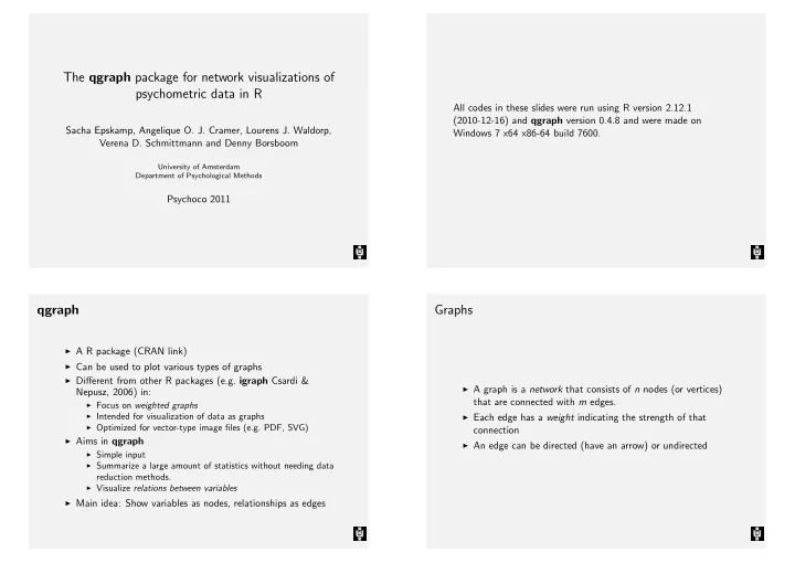
The qgraph package for network visualizations of psychometric data in R All codes in these slides were run using R version 2.12.1 (2010-12-16) and qgraph version 0.4.8 and were made on Sacha Epskamp, Angelique O. J. Cramer, Lourens J. Waldorp, Windows 7 x64 x86-64 build 7600. Verena D. Schmittmann and Denny Borsboom University of Amsterdam Department of Psychological Methods Psychoco 2011 Graphs qgraph ◮ A R package (CRAN link) ◮ Can be used to plot various types of graphs ◮ Different from other R packages (e.g. igraph Csardi & ◮ A graph is a network that consists of n nodes (or vertices) Nepusz, 2006) in: that are connected with m edges. ◮ Focus on weighted graphs ◮ Intended for visualization of data as graphs ◮ Each edge has a weight indicating the strength of that ◮ Optimized for vector-type image files (e.g. PDF, SVG) connection ◮ Aims in qgraph ◮ An edge can be directed (have an arrow) or undirected ◮ Simple input ◮ Summarize a large amount of statistics without needing data reduction methods. ◮ Visualize relations between variables ◮ Main idea: Show variables as nodes, relationships as edges

Unweighted graph Weighted graph 2 2 8 8 6 6 10 7 10 7 9 9 1 1 3 3 4 4 5 5 Weighted graph Directed graph 2 2 8 8 6 6 7 7 10 10 9 9 1 1 3 3 4 4 5 5

The qgraph() function The adjacency matrix ◮ The adj argument is the input. This can be an adjacency ◮ The main function in qgraph is qgraph() matrix ◮ Most other functions are either wrapping functions using ◮ An adjacency matrix is a square n by n matrix in which each qgraph() or functions used in qgraph() element indicates the relationship between two variables ◮ The qgraph() function requires only one argument ( adj ) ◮ Any relationship can be used as long as: ◮ A lot of other arguments can be specified, but these are all ◮ A 0 indicates no relationship ◮ Absolute negative values are similar in strength to positive optional values ◮ Examples: Usage: ◮ A 1 indicating a connection (unweighted graphs) ◮ Correlations qgraph( adj, ... ) ◮ Regression parameters ◮ Factor loadings ◮ Adjacency matrices occur naturally in statistics! Weighted graphs [,1] [,2] [,3] [1,] 0 1 1 [2,] 0 0 1 Y = η Λ T + Θ [3,] 0 0 0 > set.seed(2) 1 > eta <- matrix(rnorm(200 * 5), ncol = 5) > lam <- matrix(rnorm(50 * 5, 0, 0.15), 50, + 5) > lam[apply(diag(5) == 1, 1, rep, each = 10)] <- rnorm(50, + 0.7, 0.3) > th <- matrix(rnorm(200 * 50), ncol = 50) > Y <- eta %*% t(lam) + th 3 2

Weighted graphs Weighted graphs > cor(Y)[1:15, 1:3] > qgraph(cor(Y)) [,1] [,2] [,3] 48 49 50 1 2 [1,] 1.000000000 0.218987651 0.197325805 3 4 47 5 [2,] 0.218987651 1.000000000 0.231696634 46 6 45 7 [3,] 0.197325805 0.231696634 1.000000000 44 8 [4,] 0.464897112 0.346780772 0.279845144 43 9 10 42 [5,] 0.295912130 0.275030523 0.209220603 41 11 [6,] 0.235201044 0.272947122 0.197676521 40 12 [7,] 0.157314986 -0.001815960 -0.027551034 39 13 38 14 [8,] 0.234392422 0.212721700 0.192401237 37 15 [9,] 0.321680277 0.350685995 0.210808452 36 16 [10,] 0.204097076 0.277127339 0.148343574 35 17 [11,] -0.072734280 -0.000913891 -0.085440215 34 18 33 19 [12,] 0.052842181 0.105870583 -0.056247479 32 20 31 21 [13,] 0.001850306 0.025604291 0.081077133 30 22 29 23 28 24 [14,] -0.083391834 -0.088641129 -0.215127641 27 25 26 [15,] -0.055847218 0.007651554 0.004209916 Weighted graphs Fruchterman-Reingold layout (20 iterations) > gr <- list(1:10, 11:20, 21:30, 31:40, 41:50) > qgraph(cor(Y), groups = gr) 1 10 2 9 3 8 4 41 11 7 5 50 42 20 12 6 49 43 19 13 48 44 18 14 47 45 17 15 46 16 31 21 40 32 30 22 39 33 29 23 38 34 28 24 37 35 27 25 36 26

Fruchterman-Reingold layout (500 iterations) Saving arguments > qgraph(cor(Y), groups = gr, layout = "spring") > Q <- qgraph(cor(Y), groups = gr, layout = "spring", + minimum = 0.2) 15 15 11 17 20 37 11 24 17 20 19 37 21 27 14 24 12 19 46 18 21 27 14 16 13 29 12 25 46 18 16 13 29 30 25 49 22 44 30 28 36 48 49 23 26 22 44 28 47 36 50 48 23 26 39 32 7 43 47 50 3 39 42 32 7 43 33 3 10 6 31 42 41 35 33 5 31 40 10 6 41 35 4 5 9 40 34 38 2 4 9 34 38 1 8 2 45 1 8 45 Saving arguments Graphical arguments > Q <- qgraph(Q) > Q <- qgraph(Q, esize = 10) 15 15 11 11 17 20 17 20 37 37 24 24 19 19 21 27 21 27 14 14 12 12 46 46 18 16 18 16 13 13 29 29 25 25 30 30 49 49 22 22 28 44 28 44 36 36 48 48 23 26 23 26 47 47 50 50 39 39 32 32 7 7 43 43 3 3 42 42 33 33 10 31 10 31 6 6 41 35 41 35 5 5 40 40 4 4 9 9 34 34 38 38 2 2 1 8 1 8 45 45

Graphical arguments Graphical arguments > Q <- qgraph(Q, vsize = 4) > Q <- qgraph(Q, borders = FALSE) 15 15 11 11 17 20 17 20 37 37 24 24 19 19 21 27 14 21 27 14 12 12 46 46 18 16 18 16 29 13 29 13 25 25 30 30 49 49 22 22 28 44 28 44 36 48 36 48 23 26 23 26 47 47 50 50 39 39 32 32 7 43 7 43 3 3 42 42 33 33 10 31 10 31 6 6 41 35 41 35 5 5 40 40 4 4 9 9 34 38 34 38 2 2 1 8 1 8 45 45 Graphical arguments Graphical arguments > Q <- qgraph(Q, shape = "square") > Q <- qgraph(Q, shape = "circle") 15 15 11 11 17 20 17 20 37 37 24 24 19 19 21 27 14 21 27 14 12 12 46 46 18 18 16 16 13 13 29 29 25 25 30 30 49 49 22 22 44 44 28 28 36 36 48 48 23 26 23 26 47 47 50 50 39 39 32 32 7 43 7 43 3 3 42 42 33 33 10 6 31 10 6 31 41 35 41 35 5 5 40 40 4 4 9 9 34 38 34 38 2 2 1 1 8 8 45 45

Graphical arguments Graphical arguments > Q <- qgraph(Q, vTrans = 150) 15 11 17 20 37 24 19 21 27 14 > qgraph(Q, transparency = T, bg = T, bgcontrol = 5, 12 46 18 16 + filetype = "png", filename = "bg", res = 144, 29 13 25 + width = 7, height = 7) 30 49 22 28 44 [1] "Output stored in C:/Users/Sacha/Documents/Work/qgraph/Psych 36 48 23 26 47 50 39 32 7 43 3 42 33 10 31 6 41 35 5 40 4 9 34 38 2 1 8 45 Graphical arguments Correlations > qgraph(cor(Y), layout = "spring", groups = gr, + cut = 0.3, minimum = 0.1, maximum = 1, + graph = "association") 15 11 17 20 37 24 19 21 27 14 12 46 18 16 29 13 25 30 49 22 28 44 36 48 23 26 47 50 39 32 7 43 3 42 33 10 31 6 41 35 5 40 4 9 34 38 2 1 8 45

Partial correlations Factorial graph > qgraph(cor(Y), layout = "spring", groups = gr, > qgraph(cor(Y), layout = "spring", groups = gr, + cut = 0.3, minimum = 0.1, maximum = 1, + cut = 0.2, vsize = 2, esize = 1, borders = F, + graph = "concentration") + graph = "factorial") 38 ● 3 ● ● 10 9 ● 4 ● ● 1 2 10 50 ● ● ● 16 8 21 5 ● ● ● 6 22 12 24 35 ● 2 29 ● ● 27 30 11 46 ● 28 44 ● 17 26 ● ● 25 23 5 21 14 19 6 22 15 49 ● ● 7 16 4 32 33 47 41 42 28 29 ● ● 46 ● 20 9 42 44 43 25 ● ● ● ● 36 50 47 49 45 30 ● ● 31 41 43 ● 7 48 23 48 8 3 24 ● 38 18 27 26 40 34 ● ● 13 ● 19 33 ● 40 39 20 ● ● ● 17 34 45 31 ● ● 1 13 18 ● ● 37 ● ● ● 36 15 32 11 ● ● 39 35 ● ● 37 14 12 Factor loadings Factor loadings: EFA > qgraph.efa(cor(Y), 5, rotation = "promax", + layout = "tree", vsize = c(3, 10), groups = gr) ◮ A factor loadings matrix can be visualized using qgraph.loadings() 1 2 3 4 5 ◮ There are two wrapper functions that perform an analysis and send the results to qgraph.loadings() : ◮ qgraph.efa() performs an exploratory factor analysis (EFA) using stats:::factanal ◮ qgraph.pca() performs a principal component analysis (PCA) using psych:::principal (Revelle, 2010) ◮ These functions use a correlation or covariance matrix as input 41 42 43 44 45 46 47 48 49 50 11 12 13 14 15 16 17 18 19 20 21 22 23 24 25 26 27 28 29 30 31 32 33 34 35 36 37 38 39 40 1 2 3 4 5 6 7 8 9 10