The Power of Unbiased Recursive Partitioning: A Unifying View of - PowerPoint PPT Presentation
The Power of Unbiased Recursive Partitioning: A Unifying View of CTree, MOB, and GUIDE Lisa Schlosser, Torsten Hothorn, Achim Zeileis http://www.partykit.org/partykit Motivation 1/18 Motivation Other covariates Z 1 , . . . , Z p ? 1/18
The Power of Unbiased Recursive Partitioning: A Unifying View of CTree, MOB, and GUIDE Lisa Schlosser, Torsten Hothorn, Achim Zeileis http://www.partykit.org/partykit
Motivation 1/18
Motivation Other covariates Z 1 , . . . , Z p ? 1/18
Motivation Z j ≤ ξ Z j > ξ 1/18
Motivation M ( Y , X ; ˆ β ) Z j ≤ ξ Z j > ξ M ( Y 1 , X 1 ; ˆ M ( Y 2 , X 2 ; ˆ β 1 ) β 2 ) 1/18
Motivation M ( Y , X ; ˆ β ) Z j ≤ ξ Z j > ξ M ( Y 1 , X 1 ; ˆ M ( Y 2 , X 2 ; ˆ β 1 ) β 2 ) M can also be a more general model (possibly without X ). 1/18
Unbiased recursive partitioning GUIDE: Loh (2002, Statistica Sinica ). • First unbiased algorithm for recursive partitioning of linear models. • Separation of split variable and split point selection. • Based on χ 2 tests. CTree: Hothorn, Hornik, Zeileis (2006, JCGS ). • Proposed as unbiased recursive partitioning for nonparametric modeling. • Based on conditional inference (or permutation tests). • Can be model-based via model scores as the response transformation. MOB: Zeileis, Hothorn, Hornik (2008, JCGS ). • Model-based recursive partitioning using M-estimation (ML, OLS, CRPS, . . . ). • Based on parameter instability tests. • Adapted to various psychometric models: Rasch, PCM, Bradley-Terry, MPT, SEM, networks, . . . . 2/18
Unbiased recursive partitioning Basic tree algorithm: 1 Fit a model M ( Y , X ; ˆ β ) to the response Y and possible covariates X . 2 Assess association of M ( Y , X ; ˆ β ) and each possible split variable Z j and select the split variable Z j ∗ showing the strongest association. 3 Choose the corresponding split point leading to the highest improvement of model fit and split the data. 4 Repeat steps 1–3 recursively in each of the resulting subgroups until some stopping criterion is met. Here: Focus on split variable selection (step 2). 3/18
Split variable selection General testing strategy: 1 Evaluate a discrepancy measure capturing the observation-wise goodness of fit of M ( Y , X ; ˆ β ) . 2 Apply a statistical test assessing dependency of the discrepancy measure to each possible split variable Z j . 3 Select the split variable Z ∗ j showing the smallest p -value. Discrepancy measures: (Model-based) transformations of Y (and X , if any), possibly for each model parameter. • (Ranks of) Y . • (Absolute) deviations Y − ¯ Y . • Residuals of M ( Y , X ; ˆ β ) . • Score matrix of M ( Y , X ; ˆ β ) . • . . . 4/18
Discrepancy measures Example: Simple linear regression M ( Y , X ; β 0 , β 1 ) , fitted via ordinary least squares (OLS). Residuals: r ( Y , X , ˆ β 0 , ˆ β 1 ) = Y − ˆ β 0 − ˆ β 1 · X 5/18
Discrepancy measures Example: Simple linear regression M ( Y , X ; β 0 , β 1 ) , fitted via ordinary least squares (OLS). Residuals: r ( Y , X , ˆ β 0 , ˆ β 1 ) = Y − ˆ β 0 − ˆ β 1 · X Model scores: Based on log-likelihood or residual sum of squares. � � ∂ r 2 ( Y , X , ˆ β 0 , ˆ ∂ r 2 ( Y , X , ˆ β 0 , ˆ β 1 ) β 1 ) s ( Y , X , ˆ β 0 , ˆ β 1 ) = , ∂β 0 ∂β 1 5/18
Discrepancy measures Example: Simple linear regression M ( Y , X ; β 0 , β 1 ) , fitted via ordinary least squares (OLS). Residuals: r ( Y , X , ˆ β 0 , ˆ β 1 ) = Y − ˆ β 0 − ˆ β 1 · X Model scores: Based on log-likelihood or residual sum of squares. � � ∂ r 2 ( Y , X , ˆ β 0 , ˆ ∂ r 2 ( Y , X , ˆ β 0 , ˆ β 1 ) β 1 ) s ( Y , X , ˆ β 0 , ˆ β 1 ) = , ∂β 0 ∂β 1 ⇓ ⇓ − 2 · r ( Y , X , ˆ β 0 , ˆ − 2 · r ( Y , X , ˆ β 0 , ˆ β 1 ) β 1 ) · X 5/18
A unifying view Algorithms: CTree, MOB, GUIDE are all ‘flavors’ of the general framework. Building blocks: For standard setup. Scores Binarization Categorization Statistic CTree Model scores – – Sum of squares MOB Model scores – – Maximally selected GUIDE Residuals � � Sum of squares Remarks: • All three algorithms allow for certain modifications of standard setup. • Further differences, e.g., null distribution, pruning strategy, etc. 6/18
General framework Building blocks: • Residuals vs. full model scores. • Binarization of residuals/scores. • Categorization of possible split variables. 7/18
General framework Building blocks: • Residuals vs. full model scores. • Binarization of residuals/scores. • Categorization of possible split variables. r ( Y 1 , X 1 , ˆ β 0 , ˆ r ( Y 1 , X 1 , ˆ β 0 , ˆ β 1 ) · X 1 β 1 ) r ( Y 2 , X 2 , ˆ β 0 , ˆ r ( Y 2 , X 2 , ˆ β 0 , ˆ β 1 ) β 1 ) · X 2 s ( Y , X , ˆ β 0 , ˆ β 1 ) = − 2 · . . . . . . r ( Y n , X n , ˆ β 0 , ˆ r ( Y n , X n , ˆ β 0 , ˆ β 1 ) · X n β 1 ) 7/18
General framework Building blocks: • Residuals vs. full model scores. • Binarization of residuals/scores. • Categorization of possible split variables. r ( Y 1 , X 1 , ˆ β 0 , ˆ r ( Y 1 , X 1 , ˆ β 0 , ˆ β 1 ) · X 1 β 1 ) r ( Y 2 , X 2 , ˆ β 0 , ˆ r ( Y 2 , X 2 , ˆ β 0 , ˆ β 1 ) β 1 ) · X 2 s ( Y , X , ˆ β 0 , ˆ β 1 ) = − 2 · . . . . . . r ( Y n , X n , ˆ β 0 , ˆ r ( Y n , X n , ˆ β 0 , ˆ β 1 ) · X n β 1 ) 7/18
General framework Building blocks: • Residuals vs. full model scores. • Binarization of residuals/scores. • Categorization of possible split variables. r ( Y 1 , X 1 , ˆ β 0 , ˆ β 1 ) r ( Y 2 , X 2 , ˆ β 0 , ˆ β 1 ) r ( Y , X , ˆ β 0 , ˆ β 1 ) = . . . r ( Y n , X n , ˆ β 0 , ˆ β 1 ) 7/18
General framework Building blocks: • Residuals vs. full model scores. • Binarization of residuals/scores. • Categorization of possible split variables. r ( Y 1 , X 1 , ˆ β 0 , ˆ β 1 ) > 0 r ( Y 2 , X 2 , ˆ β 0 , ˆ β 1 ) ≤ 0 r ( Y , X , ˆ β 0 , ˆ β 1 ) = ⇒ . . . . . . r ( Y n , X n , ˆ β 0 , ˆ β 1 ) > 0 7/18
General framework Building blocks: • Residuals vs. full model scores. • Binarization of residuals/scores. • Categorization of possible split variables. Z j 1 Z j 2 Z j = . . . Z jn 7/18
General framework Building blocks: • Residuals vs. full model scores. • Binarization of residuals/scores. • Categorization of possible split variables. Z j 1 Q3 Z j 2 Q1 Z j = ⇒ . . . . . . Z jn Q2 7/18
Pruning Goal: Avoid overfitting. Two strategies: • Pre-pruning: Internal stopping criterion based on Bonferroni-corrected p -values of the underlying tests. Stop splitting when there is no significant association. • Post-pruning: First grow a very large tree and afterwards prune splits that do not improve the model fit, either via cross-validation (e.g., cost-complexity pruning as in CART) or based on information criteria (e.g., AIC or BIC). 8/18
Simulation Name Notation Specification Variables: = β 0 ( Z 1 ) + β 1 ( Z 1 ) · X + ǫ Response Y U ([ − 1 , 1 ]) Regressor X ǫ N ( 0 , 1 ) Error U ([ − 1 , 1 ]) or N ( 0 , 1 ) True split variable Z 1 U ([ − 1 , 1 ]) or N ( 0 , 1 ) Noise split variables Z 2 , Z 3 , . . . , Z 10 Parameters/functions: 0 or ± δ Intercept β 0 1 or ± δ Slope β 1 ξ ∈ { 0 , 0 . 2 , 0 . 5 , 0 . 8 } True split point ∈ { 0 , 0 . 1 , 0 . 2 , . . . , 1 } Effect size δ 9/18
Simulation 1: True tree structure varying β 0 1 z 1 ≤ ξ ● 4 z1 z 1 > ξ β 0 = +δ ● β 1 = 1 2 β 0 = −δ Y 0 ≤ ξ > ξ β 1 = 1 −2 2 3 true parameters: true parameters: −4 β 0 = 0 or −δ β 0 = 0 or +δ β 1 = 1 or +δ β 1 = 1 or −δ −1.0 −0.5 0.0 0.5 1.0 X varying β 1 varying β 0 and β 1 z 1 ≤ ξ z 1 ≤ ξ ● ● 4 4 z 1 > ξ z 1 > ξ ● ● β 0 = 0 β 0 = −δ 2 2 β 1 = +δ β 1 = +δ Y 0 Y 0 β 0 = +δ β 0 = 0 β 1 = −δ β 1 = −δ −2 −2 −4 −4 −1.0 −0.5 0.0 0.5 1.0 −1.0 −0.5 0.0 0.5 1.0 10/18 X X
Simulation 1: Residuals vs. full model scores CTree MOB GUIDE+scores GUIDE 0 0.2 0.4 0.6 0.8 1 varying β 0 varying β 1 varying β 0 and β 1 1.0 ξ = 0 (50%) 0.8 Selection probability of Z 1 0.6 0.4 0.2 0.0 1.0 ξ = 0.8 (90%) 0.8 0.6 0.4 0.2 0.0 0 0.2 0.4 0.6 0.8 1 0 0.2 0.4 0.6 0.8 1 δ 11/18
Simulation 1: Maximum vs. linear selection CTree CTree+max MOB GUIDE+scores GUIDE 0 0.2 0.4 0.6 0.8 1 varying β 0 varying β 1 varying β 0 and β 1 1.0 ξ = 0 (50%) 0.8 Selection probability of Z 1 0.6 0.4 0.2 0.0 1.0 ξ = 0.8 (90%) 0.8 0.6 0.4 0.2 0.0 0 0.2 0.4 0.6 0.8 1 0 0.2 0.4 0.6 0.8 1 δ 12/18
Simulation 1: Continuously changing parameters CTree CTree+max MOB GUIDE+scores GUIDE 0 0.2 0.4 0.6 0.8 1 varying β 0 varying β 1 varying β 0 and β 1 Selection probability of Z 1 1.0 0.8 0.6 0.4 0.2 0.0 0 0.2 0.4 0.6 0.8 1 0 0.2 0.4 0.6 0.8 1 δ 13/18
Recommend
More recommend
Explore More Topics
Stay informed with curated content and fresh updates.


