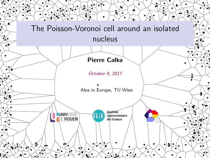
The Poisson-Voronoi cell around an isolated nucleus Pierre Calka - PowerPoint PPT Presentation

The Poisson-Voronoi cell around an isolated nucleus Pierre Calka October 9, 2017 Alea in Europe, TU Wien

default Poisson point process �� �� � � � � � � � �� �� � � � � �� �� B 4 B 1 � � � � � � � � B 2 � � B 3 � � � � � � � P λ said homogeneous Poisson point process in R 2 with intensity λ if ◮ #( P ∩ B 1 ) Poisson r.v. of mean λ A ( B 1 ) ◮ #( P ∩ B 1 ) , · · · , #( P ∩ B ℓ ) independent ( B 1 , · · · , B ℓ ∈ B ( R 2 ), B i ∩ B j = ∅ , i � = j ) Two properties D ◮ Scaling invariance: µ · P λ = P λ √ µ � � � � ◮ Mecke’s formula: E f ( x , P λ ) = λ E ( f ( x , P ∪ { x } )) d x x ∈P λ

default Poisson-Voronoi tessellation ◮ P λ homogeneous Poisson point process in R 2 of intensity λ ◮ For every nucleus x ∈ P λ , associated cell C ( x |P λ ) := { y ∈ R 2 : � y − x � ≤ � y − x ′ � ∀ x ′ ∈ P λ }

default Typical Poisson-Voronoi cell ◮ Typical cell C : chosen uniformly among all cells � 1 E ( f ( C )) = lim f ( C ( x |P λ )) a.s. r →∞ N r x ∈P λ � C ( x |P λ ) ⊂ B r ( o ) � � � 1 E ( f ( C )) = f ( C ( x |P λ ) − x ) , B ∈ B ( R 2 ) λ A ( B ) E x ∈P λ ∩ B ◮ Theorem (Slivnyak): C D = C ( o |P λ ∪ { o } ) 0

default Being in the typical cell F 0 ( K ) 0 K ◮ K convex body containing o in its interior ◮ Flower of K : F o ( K ) = ∪ x ∈ K B ( x , � x � ) Two properties ◮ Capacity probability: P ( K ⊂ C ( o |P λ ∪ { o } )) = e − λ A ( F o ( K )) ◮ Conditional distribution: ( P λ | K ⊂ C ( o |P λ ∪ { o } )) D = P λ \ F o ( K )

default The Poisson-Voronoi cell around an isolated nucleus ◮ K convex body in R 2 ◮ An origin o chosen in int ( K ) ◮ Point process ( P λ | K ⊂ C ( o |P λ ∪ { o } )) ◮ Problem 1 . Asymptotics of the characteristics of the cell K λ = C ( o |P λ ∪ { o } )

default The Poisson-Voronoi cell around an isolated nucleus o ◮ K convex body in R 2 ◮ An origin o chosen in int ( K ) ◮ Point process ( P λ | K ⊂ C ( o |P λ ∪ { o } )) ◮ Problem 1 . Asymptotics of the characteristics of the cell K λ = C ( o |P λ ∪ { o } )

default The Poisson-Voronoi cell around an isolated nucleus o ◮ K convex body in R 2 ◮ An origin o chosen in int ( K ) ◮ Point process ( P λ | K ⊂ C ( o |P λ ∪ { o } )) ◮ Problem 1 . Asymptotics of the characteristics of the cell K λ = C ( o |P λ ∪ { o } )

default The Poisson-Voronoi cell around an isolated nucleus o ◮ K convex body in R 2 ◮ An origin o chosen in int ( K ) ◮ Point process ( P λ | K ⊂ C ( o |P λ ∪ { o } )) ◮ Problem 1 . Asymptotics of the characteristics of the cell K λ = C ( o |P λ ∪ { o } )

default Two associated problems o D ⊂ R 2 , o ∈ int ( D ) Problem 2 . Cell � Problem 3 . Cell C λ ( D ) = C ( o |P λ ∪ { o } ), K λ containing K , P λ conditioned on { K ⊂ one cell } P λ conditioned on {P λ ∩ D = ∅}

default Plan Problem 1: asymptotics for K λ = C ( o |P λ \ F o ( K )) Problem 2: asymptotics for � K λ (no origin) Problem 3: asymptotics for C λ ( D ) = C ( o |P λ \ D ) Joint work with Yann Demichel (Paris Nanterre) & Nathana¨ el Enriquez (Paris-Sud)

default Plan Problem 1: asymptotics for K λ = C ( o |P λ \ F o ( K )) Context Main results Support function Rewriting of the expectations Sketch of proof Problem 2: asymptotics for � K λ (no origin) Problem 3: asymptotics for C λ ( D ) = C ( o |P λ \ D )

default Context: large Poisson-Voronoi cells ◮ Large cells in a Poisson-Voronoi tessellation: close to the circular shape D. Hug, M. Reitzner & R. Schneider (2004) ◮ When K is the unit-disk, � � � � λ →∞ λ − 2 3 2 − 1 3 − 1 3 2 2 3 − 4 1 2 2 3 π Γ 3 Γ E ( A ( K λ )) − A ( K ) ∼ , E ( N ( K λ )) λ →∞ λ ∼ 3 3 PC & T. Schreiber (2005) ◮ Estimate of the Hausdorff distance between K λ and K for a Poisson line tessellation D. Hug & R. Schneider (2014), R. Schneider (1988)

default Context: approximation of a convex body from the inside K λ = Conv( P λ ∩ K ) Efron’s relation (1965): E ( N ( K λ )) = λ ( A ( K ) − E ( A ( K λ ))) K with a smooth boundary K polygon � � � − 1 λ →∞ λ − 2 4 3 3 − 4 λ →∞ ( λ − 1 log λ ) · 2 · 3 − 1 n K A ( K ) − E ( A ( K λ )) 3 2 3 Γ 2 A ( K ) − E ( A ( K λ )) ∼ r 3 d s ∼ s 3 ∂ K A. R´ enyi & R. Sulanke (1963, 1964)

default Main results: smooth case A ( · ): area, U ( · ): perimeter, N ( · ): number of vertices r s : radius of curvature, n s : outer unit normal vector at s ∈ ∂ K � � � 1 s � s , n s � − 2 λ →∞ λ − 2 3 2 − 2 3 − 1 3 Γ 2 3 d s E ( A ( K λ )) − A ( K ) ∼ r 3 3 � � ∂ K � − 2 λ →∞ λ − 2 3 3 − 4 � s , n s � − 2 2 3 Γ E ( U ( K λ )) − U ( K ) ∼ 3 3 d s r s 3 � � ∂ K � − 2 1 1 3 2 2 3 − 4 2 3 Γ 3 d s E ( N ( K λ )) λ →∞ λ ∼ 3 � s , n s � r s 3 ∂ K

default Main results: polygonal case A ( · ): area, U ( · ): perimeter, N ( · ): number of vertices n K : number of vertices of K , { a i } : vertices of K , o i : projection of o onto ( a i , a i +1 ) o n K � � o i � − 1 λ →∞ λ − 1 2 2 − 9 3 3 2 � a i +1 − a i � E ( A ( K λ )) − A ( K ) ∼ 2 π 2 2 i =1 λ →∞ ( λ − 1 log λ ) · 2 − 1 3 − 1 � n K i =1 � o i � − 1 E ( U ( K λ )) − U ( K ) ∼ λ →∞ (log λ ) · 2 · 3 − 1 n K . E ( N ( K λ )) ∼

default Support function p o ( K , θ ) u θ K o Support function � x , u θ � p o ( K , θ ) = p o ( K , u θ ) = sup x ∈ K with u θ = (cos( θ ) , sin( θ )) Two properties ◮ Link with the flower: sup { r > 0 : ru θ ∈ F o ( K ) } = 2 p o ( K , θ ) � 2 π ◮ Cauchy-Crofton formula: U ( K ) = p o ( K , θ ) d θ 0

default Rewriting of the expectations ◮ Mean defect area � E ( A ( K λ )) − A ( K ) = P ( x ∈ K λ ) d x R 2 \ K � e − λ ( A ( F o ( K ∪{ x } )) −A ( F o ( K ))) d x = R 2 \ K � 2 π p o ( K , θ ) 2 d θ where A ( F o ( K )) = 2 0 ◮ Mean defect perimeter � 2 π E ( U ( K λ )) − U ( K ) = E ( p o ( K λ , θ ) − p o ( K , θ )) d θ 0 ◮ Mean number of vertices: Efron-type relation E ( N ( K λ )) = λ ( E ( A ( F o ( K λ )) − A ( F o ( K ))) � 2 π λ →∞ 4 λ ∼ p o ( K , θ ) E ( p o ( K λ , θ ) − p o ( K , θ )) d θ 0

default Sketch of proof, smooth case 1 2 @ F o ( K ) z ( s ) n s s 1 2 s n s @K o − 1 3 9 2 2 2 3 − 1 r A ( F o ( K ∪ { s + hn s } )) − A ( F o ( K )) ∼ h → 0 h 2 � s , n s � s

default Sketch of proof, smooth case osculating circle of 1 2 @ F o ( K ) 2 @ F o ( K ) 1 α s z 00 ( s ) z 0 ( s ) k s k 2 ρ z ( s ) = h 2 k s k� r s cos α s z ( s ) s + hn s h α s n s s α s 1 2 ( s + hn s ) 1 2 s n s @K o − 1 3 9 2 2 2 3 − 1 r A ( F o ( K ∪ { s + hn s } )) − A ( F o ( K )) ∼ h → 0 h 2 � s , n s � s

default Sketch of proof, smooth case n s m s,λ Y s,λ t s s X s,λ ∂K o ◮ m s ,λ : support point of K λ in direction n s ◮ ( X s ,λ , Y s ,λ ): coordinates of m s ,λ in the Frenet frame at s 1 3 Y s ,λ ) D 2 3 X s ,λ , λ ( λ → ( X , Y ) with explicit density. � 2 � 1 λ →∞ λ − 2 3 3 − 4 s � s , n s � − 2 3 Γ E ( p o ( K λ , n s ) − p o ( K , n s )) = E ( Y s ,λ ) ∼ 3 r 3 3

default Problem 2: asymptotics for � K λ (no origin) ◮ Steiner point � 2 π st( K ) = 1 p o ( K , θ ) u θ d θ = argmin x A ( F x ( K )) π 0 ◮ K : convex body with Steiner point at o ◮ � K λ : cell containing K , conditional on S λ = { K ⊂ one cell } ◮ Z λ : nucleus of � K λ 1 D → N ( o , (4 π ) − 1 I 2 ). Conditional on S λ , λ 2 Z λ The expectation asymptotics of � K λ coincide with those of K λ when o = st( K ).

default Problem 3: asymptotics for C λ ( D ) = C ( o |P λ \ D ) D K o ◮ D closed domain, o ∈ int( D ) ◮ C λ ( D ) = C ( o |P λ \ D ) ◮ K : convex body such that F o ( K ) is the largest flower in D ◮ D ∗ : maximal starlike set in D , with piecewise C 3 equation d ( · ) C λ ( D ) P → K in the Hausdorff metric � � � λ →∞ λ − 2 3 2 − 8 3 3 − 1 4 3 d ( θ ) − 2 3 Γ 2 ( d ( θ ) + d ′′ ( θ )) E ( A ( C λ ( D ))) − A ( K ) ∼ 3 d θ 3 � � � λ →∞ λ − 2 3 2 − 2 3 3 − 4 1 3 d ( θ ) − 2 2 3 Γ ( d ( θ ) + d ′′ ( θ )) E ( U ( C λ ( D ))) − U ( K ) ∼ 3 d θ 3 � � � 1 3 2 − 8 3 3 − 4 1 1 2 3 Γ ( d ( θ ) + d ′′ ( θ )) E ( N ( C λ ( D ))) ∼ 3 d ( θ ) 3 d θ λ →∞ λ 3

default Problem 3: asymptotics for C λ ( D ) = C ( o |P λ \ D )

default Concluding remarks ◮ Higher dimension ◮ Variances ◮ Similar results for the zero-cell of a Poisson line tessellation ◮ Inlets

default Concluding remarks

default Concluding remarks

default Concluding remarks

default Thank you for your attention!