The PLS approach to Generalised Linear Models and Causal Path - PDF document

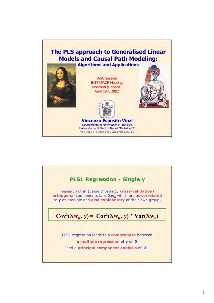
The PLS approach to Generalised Linear Models and Causal Path Modeling: Algorithms and Applications IASC Session INTERFACE Meeting Montreal (Canada) April 19 th , 2002 Vincenzo Esposito Vinzi Dipartimento di Matematica e Statistica Università degli Studi di Napoli “Federico II” vincenzo.espositovinzi@unina.it 1 PLS1 Regression - Single y Research of m (value chosen by cross-validation ) orthogonal components t h = Xw h which are as correlated to y as possible and also explanatory of their own group . Cov 2 (Xw h , y) = Cor 2 (Xw h , y) * Var(Xw h ) PLS1 regression leads to a compromise between a multiple regression of y on X and a principal component analysis of X . 2 1

A new presentation of PLS1 in terms of OLS simple and multiple regressions 1. The m-components PLS regression model ( non linear in the parameters) may be written as :   p m ∑ ∑ = * + y c w x residual   h hj j   = = h 1 j 1 with the orthogonality constraints on the PLS components . 2. The first PLS component is defined as: 1 p ( ) ∑ = × t cov y x , x 1 j j p ( ) ∑ = j 1 2 cov y x , j = j 1 3 A new presentation of PLS1 in terms of OLS simple and multiple regressions 3. The covariance is also the regression coefficient ( a 1j ) in the OLS simple regression between y and x j /var( x j ): ( ) ( ) = + + y a a x var x ε 0 j 1 j j j In fact:   1   cov y , x ( )   j var x   ( ) j = = a cov y x , 1 j   j 1   var x ( )   j var x   j 4. A test on the regression coefficient ( a 1j ) evaluates the importance of variable x j in building up t 1 . Non significant covariances are set to 0. 4 2

A new presentation of PLS1 in terms of OLS simple and multiple regressions 5. For the computation of the second PLS component , we first deflate y and x j ’s with respect to t 1 : = + y c t y 1 1 1 = + x p t x j 1 j 1 1 j and then we define t 2 as: p 1 ( ) ∑ = × t cov y x , x 2 1 1 j 1 j p ( ) ∑ = j 1 2 cov y x , 1 1 j = j 1 6. Because of the orthogonality between residual x 1j and component t 1 , the covariance is now the regression coefficient in the following OLS multiple regression : ( ) ( ) = + + y c t a x var x residual 1 1 2 j 1 j 1 j 5 A new presentation of PLS1 in terms of OLS simple and multiple regressions 7. Partial correlation between y and x j conditioned to t 1 is defined as the correlation between residuals y 1 and x 1j . The same applies to partial covariance: ( ) ( ) = cov y x , | t cov y x , j 1 1 1 j leading to: 1 p ( ) ∑ = × t cov y x , | t x 2 j 1 1 j p ( ) ∑ j = 1 2 cov y x , | t j 1 = j 1 8. Since ( t 1 , x 1j ) and ( t 1 , x j ) span the same space, the contribution of variable x j to the construction of t 2 is finally tested by means of the following OLS multiple regression : = + + + y d d t d x ε 0 j 1 j 1 2 j j Non significant covariances are set to 0. 6 3

A new presentation of PLS1 in terms of OLS simple and multiple regressions 9. The second PLS compoent t 2 may be well expressed as a function of the original variables (namely, those retained for t 1 and those significant for t 2 ) because the residuals x 1j are expressed as functions of the original variable x j : = − x x p t 1 j j 1 j 1 10. The procedure STOP s when all partial covariances become non significant . 7 PLS for Logistic Regression Bordeaux Wine Dataset Variables observed in 34 years (1924 - 1957) Meteorological Variables (covariates) - standardised • TEMPERATURE : Sum of daily mean temperatures (°C) • SUNSHINE : Duration of sunshine (hours) • HEAT : Number of very warm days • RAIN : Rain height (mm) Ordinal Response Variable (three categories) • QUALITY of WINE: 1=Good, 2=Average, 3=Poor 8 4

The Dataset Bordeaux Wine Obs Obs Obs Obs Year Temperature Sunshine Heat Rain Quality Year Temperature Sunshine Heat Rain Quality Year Temperature Sunshine Heat Rain Quality Year Temperature Sunshine Heat Rain Quality 1 1924 3064 1201 10 361 2 2 1925 3000 1053 11 338 3 3 1926 3155 1133 19 393 2 4 1927 3085 970 4 467 3 5 1928 3245 1258 36 294 1 6 1929 3267 1386 35 225 1 7 1930 3080 966 13 417 3 8 1931 2974 1189 12 488 3 9 1932 3038 1103 14 677 3 10 1933 3318 1310 29 427 2 11 1934 3317 1362 25 326 1 12 1935 3182 1171 28 326 3 13 1936 2998 1102 9 349 3 14 1937 3221 1424 21 382 1 15 1938 3019 1230 16 275 2 16 1939 3022 1285 9 303 2 17 1940 3094 1329 11 339 2 18 1941 3009 1210 15 536 3 19 1942 3227 1331 21 414 2 20 1943 3308 1366 24 282 1 21 1944 3212 1289 17 302 2 22 1945 3361 1444 25 253 1 23 1946 3061 1175 12 261 2 24 1947 3478 1317 42 259 1 25 1948 3126 1248 11 315 2 26 1949 3458 1508 43 286 1 27 1950 3252 1361 26 346 2 28 1951 3052 1186 14 443 3 29 1952 3270 1399 24 306 1 30 1953 3198 1259 20 367 1 31 1954 2904 1164 6 311 3 32 1955 3247 1277 19 375 1 9 33 1956 3083 1195 5 441 3 34 1957 3043 1208 14 371 3 Classical Ordinal Logistic Regression y = Quality : Good (1), Average (2), Poor (3) Proportional Odds Ratio Model ≤ l l ) = l l PROB(y ≤ ≤ ≤ α + β + β + β + β Temperature Sunshine Heat Rain e � 1 2 3 4 + α + β + β + β + β Temperature Sunshine Heat Rain 1 e � 1 2 3 4 10 5

Ordinal Logistic Regression SAS Results (Proc LOGISTIC) Score Test for the Proportional Odds Assumption Model with equal slopes Chi-Square = 2.9159 with 4 DF (p=0.5720) is acceptable Analysis of Maximum Likelihood Estimates Parameter Standard Wald Pr > Variable DF Estimate Error Chi-Square Chi-Square INTERCP1 1 -2.6638 0.9266 8.2641 0.0040 INTERCP2 1 2.2941 0.9782 5.4998 0.0190 TEMPERA 1 3.4268 1.8029 3.6125 0.0573 SUN 1 1.7462 1.0760 2.6335 0.1046 HEAT 1 -0.8891 1.1949 0.5536 0.4568 RAIN 1 -2.3668 1.1292 4.3931 0.0361 Significant at Uncoherent Sign 10% risk level 11 Ordinal Logistic Regression Model Prediction Performance OBSERVED PREDICTION QUALITY Frequency‚ 1‚ 2‚ 3‚ Total ƒƒƒƒƒƒƒƒƒˆƒƒƒƒƒƒƒƒˆƒƒƒƒƒƒƒƒˆƒƒƒƒƒƒƒƒˆ 1 ‚ 8 ‚ 3 ‚ 0 ‚ 11 ƒƒƒƒƒƒƒƒƒˆƒƒƒƒƒƒƒƒˆƒƒƒƒƒƒƒƒˆƒƒƒƒƒƒƒƒˆ 2 ‚ 2 ‚ 8 ‚ 1 ‚ 11 ƒƒƒƒƒƒƒƒƒˆƒƒƒƒƒƒƒƒˆƒƒƒƒƒƒƒƒˆƒƒƒƒƒƒƒƒˆ 3 ‚ 0 ‚ 1 ‚ 11 ‚ 12 ƒƒƒƒƒƒƒƒƒˆƒƒƒƒƒƒƒƒˆƒƒƒƒƒƒƒƒˆƒƒƒƒƒƒƒƒˆ Total 10 12 12 34 Result: 7 (20.6%) years are misclassified 12 6

Ordinal Logistic Regression Problems for Interpretation • Not significant coefficients for some covariates that are known to be influent • Uncoherent signs for some coefficients • High percentage of misclassified observations Multicollinearity between covariates 13 Covariates Correlation Matrix Temperature Sunshine Heat Rain Temperature Sunshine Heat Rain Temperature Sunshine Heat Rain Temperature Sunshine Heat Rain Temperature 1.00000 0.71235 0.86510 -0.40962 Temperature Temperature Temperature Sunshine Sunshine Sunshine Sunshine 0.71235 1.00000 0.64645 -0.47340 Heat Heat Heat Heat 0.86510 0.64645 1.00000 -0.40114 Rain Rain Rain Rain -0.40962 -0.47340 -0.40114 1.00000 Quite strong correlations between Temperature, Heat and Sunshine 14 7