The Normalization Shortcut stands for the probability distribution - PDF document
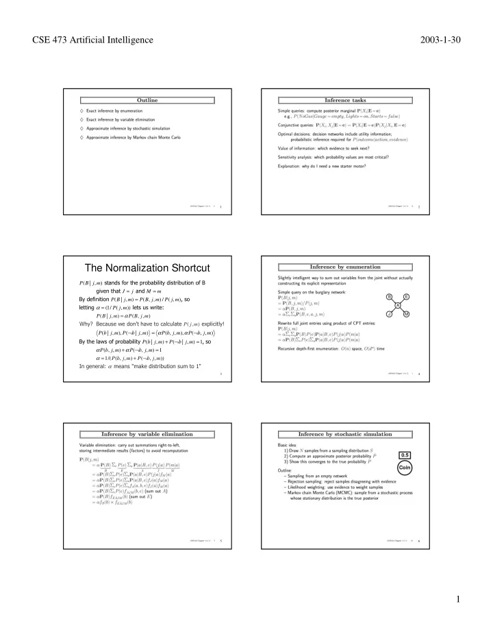
CSE 473 Artificial Intelligence 2003-1-30 1 2 The Normalization Shortcut stands for the probability distribution of B ( | , ) P B j m given that and J = j M = m By definition , so P B j m ( | , ) = P B j m ( , , ) / P j m
CSE 473 Artificial Intelligence 2003-1-30 1 2 The Normalization Shortcut stands for the probability distribution of B ( | , ) P B j m given that and J = j M = m By definition , so P B j m ( | , ) = P B j m ( , , ) / P j m ( , ) letting lets us writ e : α = (1/ P j ( , m )) ( | , ) = α ( , , ) P B j m P B j m Why? Because we don't have t o calculate explicitly! ( , ) P j m ( | , ), ( ¬ | , ) = α ( , , ), α ( ¬ , , ) P b j m P b j m P b j m P b j m By the laws of probability , so ( | , ) + ( ¬ | , ) = 1 P b j m P b j m α ( , , ) + α ( ¬ , , ) = 1 P b j m P b j m α = 1/( ( , , P b j m ) + P ( ¬ b j m , , ) ) In general: means "make distr ibut ion sum to 1" α 3 4 5 6 1
CSE 473 Artificial Intelligence 2003-1-30 7 8 9 10 11 12 2
CSE 473 Artificial Intelligence 2003-1-30 13 14 15 16 Markov Chain Monte Carlo MCMC with Gibbs Sampling Fix the values of observed variables Set the values of all non-observed variables randomly Perform a random walk through the space of complete variable assignments. On each move: 1. Pick a variable X 2. Calculate Pr(X=true | all other variables) 3. Set X to true with that probability Repeat many times. Frequency with which any variable X is true is it’s posterior probability. Converges to true posterior when frequencies stop changing significantly • stable distribution, mixing CSE 592 17 CSE 592 18 3
CSE 473 Artificial Intelligence 2003-1-30 Markov Blanket Sampling Example How to calculate Pr(X=true | all other variables) ? ∏ P X ( ) = α P X Parents X ( | ( )) P Y Parents Y ( | ( )) Recall: a variable is independent of all others given it’s Y Children X ∈ ( ) Markov Blanket • parents ( , , , ) A P X A B C ( | , , ) = P X A B C • children P A B C ( , , ) • other parents of children P A P X A P C P B ( ) ( | ) ( ) ( | X , C ) C So problem becomes calculating Pr(X=true | MB(X)) X = P A B ( , , C ) • We solve this sub-problem exactly • Fortunately, it is easy to solve ( ) ( ) P A P C = P X A P B X C ( | ) ( | , ) B ∏ P A B C ( , , ) ( ) = α ( | ( )) ( | ( )) P X P X Parents X P Y Parents Y ∈ ( ) Y Children X = α ( | ) ( | , ) P X A P B X C CSE 592 19 CSE 592 20 Example Example 2 P(s) P(s) 0.2 0.2 S P(l) S P(l) smoking smoking T 0.8 T 0.8 F 0.1 F 0.1 S P(s) S P(h) T 0.6 T 0.6 heart heart lung lung F 0.1 F 0.1 disease disease disease disease Evidence: Evidence: S=true, B=true S=true, B=true shortness shortness Randomly set H=false, L=true of breath of breath H L P(b) H L P(b) T T 0.9 T T 0.9 T F 0.8 T F 0.8 F T 0.7 F T 0.7 F F 0.1 F F 0.1 CSE 592 21 CSE 592 22 Example 3 Example 4 P(s) P(s) 0.2 0.2 S P(l) S P(l) smoking smoking T 0.8 T 0.8 F 0.1 F 0.1 S P(h) S P(h) T 0.6 T 0.6 heart heart lung lung F 0.1 F 0.1 disease disease disease disease Sample H: Sample L: P(h|s,l,b)= α P(h|s)P(b|h,l) P(l|s,h,b)= α P(l|s)P(b|h,l) shortness shortness = α (0.6)(0.9)= α 0.54 = α (0.8)(0.9)= α 0.72 of breath of breath H L P(b) H L P(b) P( ¬ h|s,l,b)= α P( ¬ h|s)P(b| ¬ h,l) P( ¬ l|s,h,b)= α P( ¬ l|s)P(b| h, ¬ l) T T 0.9 T T 0.9 = α (0.4)(0.7)= α 0.28 = α (0.2)(0.8)= α 0.16 T F 0.8 T F 0.8 Normalize: 0.54/(0.54+0.28)=0.66 Normalize: 0.72/(0.72+0.16)=0.82 F T 0.7 F T 0.7 Flip coin: H becomes true (maybe) Flip coin: … F F 0.1 F F 0.1 CSE 592 23 CSE 592 24 4
CSE 473 Artificial Intelligence 2003-1-30 Example 5: Different Evidence Example 6 P(s) P(s) 0.2 0.2 S P(l) S P(l) smoking smoking T 0.8 T 0.8 F 0.1 F 0.1 S P(s) S P(h) T 0.6 T 0.6 heart heart lung lung F 0.1 F 0.1 disease disease disease disease Evidence: Evidence: S=true, B=false S=true, B=false shortness shortness Randomly set H=false, L=true of breath of breath H L P(b) H L P(b) T T 0.9 T T 0.9 T F 0.8 T F 0.8 F T 0.7 F T 0.7 F F 0.1 F F 0.1 CSE 592 25 CSE 592 26 Example 7 Example 8 P(s) P(s) 0.2 0.2 S P(l) S P(l) smoking smoking T 0.8 T 0.8 F 0.1 F 0.1 S P(h) S P(h) T 0.6 T 0.6 heart heart lung lung F 0.1 F 0.1 disease disease disease disease Sample H: Sample L: P(h|s,l, ¬ b)= α P(h|s)P( ¬ b|h,l) P(l|s, ¬ h, ¬ b)= α P(l|s)P( ¬ b| ¬ h,l) shortness shortness = α (0.6)(0.1)= α 0.06 = α (0.8)(0.3)= α 0.24 of breath of breath H L P(b) H L P(b) P( ¬ h|s,l, ¬ b)= α P( ¬ h|s)P( ¬ b| ¬ h,l) P( ¬ l|s, ¬ h, ¬ b)= α P( ¬ l|s)P( ¬ b| ¬ h, ¬ l) T T 0.9 T T 0.9 = α (0.4)(0.3)= α 0.12 = α (0.2)(0.9)= α 0.18 T F 0.8 T F 0.8 Normalize: 0.06/(0.06+0.12)=0.33 Normalize: 0.24/(0.24+0.18)=0.75 F T 0.7 F T 0.7 F F 0.1 Flip coin: H stays false (maybe) F F 0.1 Flip coin: … CSE 592 27 CSE 592 28 (and rejection sampling) 29 30 5
CSE 473 Artificial Intelligence 2003-1-30 31 32 33 34 35 36 6
CSE 473 Artificial Intelligence 2003-1-30 37 38 A survey & taxonomy of location technologies The Location Stack: Design and Sensor-Fusion for Ad hoc signal strength Physical contact GPS DC magnetic pulses Cellular E-911 Location-Aware Ubicomp Jeffrey Hightower Infrared proximity Ultrasonic time of flight Laser range-finding Stereo vision 39 40 [Hightower and Borriello, IEEE Computer , Aug 2001] 39 40 Principle 4: Applications are The Location Stack concerned with activities . 5 Principles Intentions Intentions • Dinner is in progress. 1. There are fundamental Activities Activities measurement techniques . • A presentation is going on in Mueller 153. 2. There are standard ways Contextual Fusion Contextual Fusion • Jeff is walking through his house listening to combine measurements . to The Beatles. Arrangements Arrangements Non Non- - 3. There are standard object Location Location • Jane is dispensing ethylene-glycol into relationship queries . Fusion Fusion Context Context 4. Applications are beaker #45039. Abstractions Abstractions Measurements Measurements concerned with activities . • Elvis has left the building. 5. Uncertainty is important . Sensors Sensors 41 42 [Hightower, Brumitt, and Borriello, WMCSA , Jan 2002] 41 42 7
CSE 473 Artificial Intelligence 2003-1-30 Principle 5: Uncertainty is Fusion using Monte Carlo localization important . (MCL) ( | ) p m x Example: routing phone calls to nearest handset Bel (x) Bel (x) x x ( t = ) ( | ... ) Bel x p x m m 0 t t ∫ ( ) = η ( | ) ( | ) ( ) Bel x p m x p x x Bel x dx t t t t t − 1 t − 1 t − 1 X X p ( m | x ) Bel (x) Bel (x) x x 43 44 [Hightower and Borriello, Ubicomp LMUC Workshop , Sep 2001] 43 44 MCL details 2D MCL Example: Robocup Motion models: ( | ) p x t x t − 1 • 1 Object • 2 types of Stochastically shift t+1 t+2 Measurements all particles Vision marker distance Odometry • Red dot is most likely ( | ) Sensor likelihood models: p m t x t state. (x,y,orientation) probability R B distance 45 46 [Fox et al., Sequential Monte Carlo Methods in Practice , 2000] 45 46 Adaptive MCL Location Stack Implementation World Map • Performance improvement: adjust sample Service MCL-based count to best represent the posterior. Fusion 1. Assume we know the true Bel(x) represented Engine(s) Hierarchical as a multinomial distribution. Object 2. Determine number of samples such that with Relationship Database probability ( 1-p) , the Kullback-Leibler distance between the true posterior and the Sensor Driver Sensor Driver Sensor Driver particle filter representation is less than ε Sensor Sensor Sensor Hardware Hardware Hardware 47 48 [Fox, NIPS , 2002] 47 48 8
CSE 473 Artificial Intelligence 2003-1-30 Location Stack Supported The Location Stack in action Technologies 1. VersusTech commercial infrared badge proximity system 2. RF Proximity using the Berkeley motes 3. SICK LMS-200 180º infrared laser range finders 4. MIT Cricket ultrasound range beacons 5. Indoor harmonic radar, in progress 6. 802.11b WiFi triangulation system, in progress 7. Cellular telephone E-OTD, planned 49 50 49 50 Person Tracking with Anonymous Person Tracking with Anonymous and Id-Sensors: Motivation and Id-Sensors: Concept • Accurate anonymous sensors exist • Use Rao-Blackwellised particle filters to efficiently estimate locations • Id-sensors are less accurate but provide 1. Each particle is an association history between explicit object identity information. Kalman filter object tracks and observations. 2. Due to initial id uncertainty, starts by tracking using only anonymous sensors and estimating object id's with sufficient statistics. 3. Once id estimates are certain enough, sample id them using a fully Rao-Blackwellised particle filter over both object tracks and id assignments. 51 52 [Fox, Hightower, and Schulz., Submitted to IJCAI , 2003] 51 52 Experimental Setup Experimental Setup 53 54 53 54 9
Recommend
More recommend
Explore More Topics
Stay informed with curated content and fresh updates.


