The Mathematics of Quatrainment Finding the Solution Loran Briggs - - PowerPoint PPT Presentation

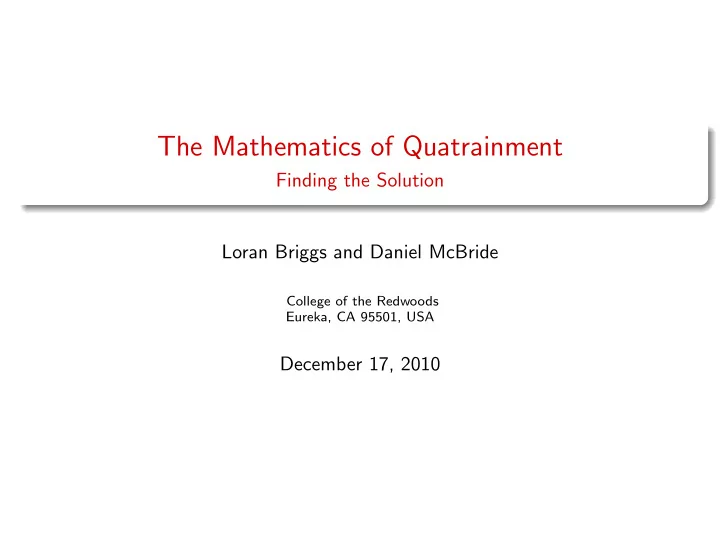
The Mathematics of Quatrainment

Finding the Solution Loran Briggs and Daniel McBride

College of the Redwoods Eureka, CA 95501, USA

December 17, 2010

Abstract

The game of Quatrainment is a simple game where you flip over tiles to make a 4 by 4 gird look like another target 4 by 4 grid. This is an example of a finite-state machine. In this presentation, we will be discussing our method of finding a unique solution to any quatrainment game using the fewest number

• f moves possible. We will go through the rules of the game, figuring out

whether or not there is a solution to every game, how to find a solution, as well as our program which finds the quickest solution to the game.

Loran Briggs and Daniel McBride (CR) The Mathematics of Quatrainment December 17, 2010 2 / 19

Overview

Setup and Goal Rules Base Two Systems Is a Solution Always Possible? The Solution Algorithm

Loran Briggs and Daniel McBride (CR) The Mathematics of Quatrainment December 17, 2010 3 / 19

Setup and Goal

Starting Grid X X X X X X X Target Grid X X X X X X X

Loran Briggs and Daniel McBride (CR) The Mathematics of Quatrainment December 17, 2010 4 / 19

Rules

Corner Cell Selected. Inner Cell Selected Edge Cell Selected

Loran Briggs and Daniel McBride (CR) The Mathematics of Quatrainment December 17, 2010 5 / 19

Base Two System

Four possibilities when adding in base two: 0 + 0 = 0 0 + 1 = 1 1 + 0 = 1 1 + 1 = 0 1 1 1 1 1 1 1 + 1 1 1 1 1 1 = 1 1 1 1 1 1 1 1 1

Loran Briggs and Daniel McBride (CR) The Mathematics of Quatrainment December 17, 2010 6 / 19

Is a Solution Always Possible?

First we need to define our moves in the form of 4 × 4 matrices. M1 = 1

1 1 1 1 1

• M2 =

1

1 1

• M3 =

1 1 1

• M4 =

1 1 1 1 1 1

• M5 =

1

1 1

• M6 =

1 1 1 1 1

• M7 =

1 1 1 1 1

• M8 =

1 1 1

• M9 =

1 1 1

• M10 =

1 1 1 1 1

• M11 =

1 1 1 1 1

• M12 =

1 1 1

• M13 =

1 1 1 1 1 1

• M14 =

1 1 1

• M15 =

1 1 1

• M16 =

1 1 1 1 1 1

• Loran Briggs and Daniel McBride (CR)

The Mathematics of Quatrainment December 17, 2010 7 / 19

Are the Inputs Linearly Independent?

Is every target array reachable from any starting array? Are the input moves independent of each other? α1M1 + α2M2 + α3M3 + α4M4 + α5M5 + α6M6 + α7M7 + α8M8 + α9M9+ α10M10 + α11M11 + α12M12 + α13M13 + α14M14 + α15M15 + α16M16 = 0 Is the only solution the trival solution? α0 = α1 = α2 = α3 = α4 = α5 = α6 = α7 = α8 = α9 = α10 = α11 = α12 = α13 = α14 = α15 = α16 = 0

Loran Briggs and Daniel McBride (CR) The Mathematics of Quatrainment December 17, 2010 8 / 19

To do this we expand our Mi matrices and multiply them with our α′s which gives     α1 α1 α1 α1 α1 α1     +     α2 α2 α2     +     α3 α3 α3     +     α4 α4 α4 α4 α4 α4     +     α5 α5 α5     +     α6 α6 α6 α6 α6     + · · · +     α16 α16 α16 α16 α16 α16     =        

Loran Briggs and Daniel McBride (CR) The Mathematics of Quatrainment December 17, 2010 9 / 19

Each cell indiviually must equal zero, form the zero matrix α1 + α2 + α5 = 0 α1 + α3 + α4 + α6 = 0 α1 + α2 + α4 + α7 = 0 α3 + α4 + α8 = 0 α1 + α6 + α9 + α13 = 0 α2 + α5 + α6 + α7 + α10 = 0 α3 + α4 + α6 + α7 + α8 + α11 = 0 α4 + α7 + α12 + α16 = 0 α1 + α5 + α10 + α13 = 0 α6 + α9 + α10 + α11 + α13 + α14 = 0 α7 + α10 + α11 + α12 + α15 + α16 = 0 α4 + α8 + α11 + α16 = 0 α9 + α13 + α14 = 0 α10 + α13 + α15 + α16 = 0 α11 + α13 + α14 + α16 = 0 α12 + α15 + α16 = 0

Loran Briggs and Daniel McBride (CR) The Mathematics of Quatrainment December 17, 2010 10 / 19

The previous sixteen equations form this matrix here. Rα = 0 :                             1 1 1 1 1 1 1 1 1 1 1 1 1 1 1 1 1 1 1 1 1 1 1 1 1 1 1 1 1 1 1 1 1 1 1 1 1 1 1 1 1 1 1 1 1 1 1 1 1 1 1 1 1 1 1 1 1 1 1 1 1 1 1 1 1 1 1 1                                                         α1 α2 α3 α4 α5 α6 α7 α8 α9 α10 α11 α12 α13 α14 α15 α16                             =                                                        

Loran Briggs and Daniel McBride (CR) The Mathematics of Quatrainment December 17, 2010 11 / 19

In reduced row echelon form, matrix R yeilds:                             1 1 1 1 1 1 1 1 1 1 1 1 1 1 1 1                             Since there is a pivot in every row, R is non-singular and therefore our input moves are linearly independent.

Loran Briggs and Daniel McBride (CR) The Mathematics of Quatrainment December 17, 2010 12 / 19

The Solution Algorithm

If we replace the zero vector from before with a target vector we call p. We can now take our equation: Rα = p Solving for α gives R−1Rα =R−1p α =R−1p Now to find R−1.

Loran Briggs and Daniel McBride (CR) The Mathematics of Quatrainment December 17, 2010 13 / 19

Using a MATLAB program named bin_solve, we have our R−1 R−1 =                             1 1 1 1 1 1 1 1 1 1 1 1 1 1 1 1 1 1 1 1 1 1 1 1 1 1 1 1 1 1 1 1 1 1 1 1 1 1 1 1 1 1 1 1 1 1 1 1 1 1 1 1 1 1 1 1 1 1 1 1 1 1 1 1 1 1 1 1 1 1 1 1 1 1 1 1 1 1 1 1 1 1 1 1 1 1 1 1 1 1 1 1 1 1 1 1 1 1 1 1 1 1 1 1 1 1 1 1 1 1 1 1 1 1 1 1                            

Loran Briggs and Daniel McBride (CR) The Mathematics of Quatrainment December 17, 2010 14 / 19

So now we take our initial matrix and our final matrix add them together to get

• ur matrix P, we convert our P matrix into a vector p. We then find our α by

α = R−1p For example: X X X X X X X Initial Grid X X X X X X X Target Grid

Loran Briggs and Daniel McBride (CR) The Mathematics of Quatrainment December 17, 2010 15 / 19

We wrote a program in MATLAB which will help us. First we convert our grids to base 2 matrices. 1 1 1 1 1 1 1 1 1 1 1 1 1 1 Add them together to get: 1 1 1 1 This is our P matrix

Loran Briggs and Daniel McBride (CR) The Mathematics of Quatrainment December 17, 2010 16 / 19

We then convert our P matrix into the vector p on the left. p =                             1 1 1 1                             α = R−1p =                             1 1 1 1 1 1 1 1                             Now, using MATLAB we multiply R−1p to get our α on the right.

Loran Briggs and Daniel McBride (CR) The Mathematics of Quatrainment December 17, 2010 17 / 19

We then convert our α back into the following matrix:     1 1 1 1 1 1 1 1    

Loran Briggs and Daniel McBride (CR) The Mathematics of Quatrainment December 17, 2010 18 / 19

QUESTIONS?

Loran Briggs and Daniel McBride (CR) The Mathematics of Quatrainment December 17, 2010 19 / 19