The magic of cross-spectrum measurements from DC to optics E. - PowerPoint PPT Presentation

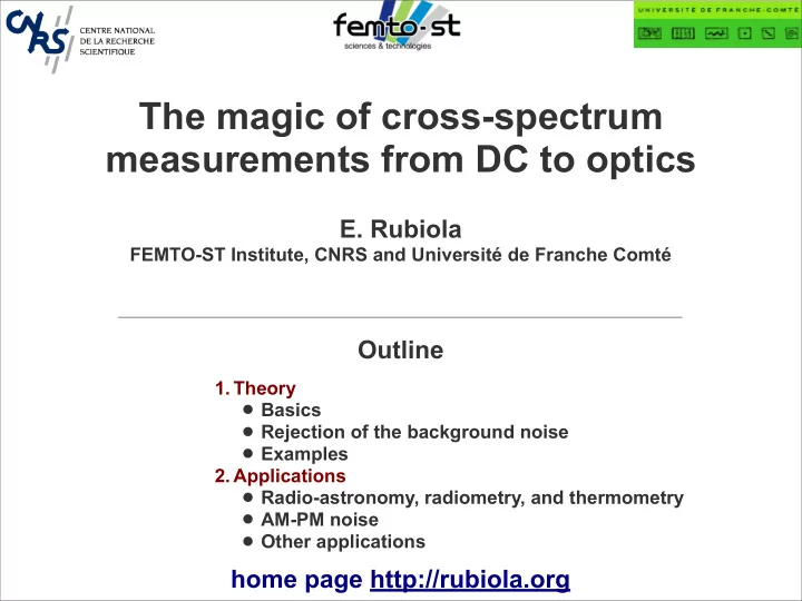
The magic of cross-spectrum measurements from DC to optics E. Rubiola FEMTO-ST Institute, CNRS and Université de Franche Comté Outline 1. Theory • Basics • Rejection of the background noise • Examples 2. Applications • Radio-astronomy, radiometry, and thermometry • AM-PM noise • Other applications home page http://rubiola.org

2 Part 1 – Theory

3 The main idea Instrument A x = a + c Σ CORRELATOR instr. a ( t ) noise c ( t ) DUT input Instrument B signal y = b + c Σ instr. b ( t ) noise • Two instruments measure independently the same physical quantity • Averaging must help to reject the instrument noise, and measure the statistical properties of the signal Notation: Fourier transform x(t) <=> X(ıf) = X’(ıf)+ ıX”(ıf)

4 Ergodicity FFT => sequence of discrete spectra spectra seq. analog sample no B d , S S(f) S j (f) S jk integer time integer frequency time j lock j=J & run k: S Jk is a spectrum k y c n run j & lock k=K: S jK is a time series e u q e r f white noise: S(f 1 ) and S(f 2 ), f 1 ≠ f 2 , are uncorrelated, hence given i, S k can be seen as the ensemble (at a given time) Ergodicity allows to interchange time-statistics with ensemble statistics. Sweeping the frequency, we get the statistical behavior of the time series. No need for forthcoming samples. Useful when S is a large-size average. flicker noise: need f 1 ≠≠ f 2 , for S(f 1 ) and S(f 2 ), to be uncorrelated (less deg. of freedom)

5 Single-channel spectrum Sxx gaussian X with independent Re and Im Spectrum � S xx � m = � XX ∗ � m = � ( X ′ + ıX ′′ ) × ( X ′ − ıX ′′ ) � m ( X ′ ) 2 + ( X ′′ ) 2 � � = m white, gaussian, avg = 0, var = 1/2 white, χ 2 , with 2m degrees of freedom avg = 1, var = 1/m � the S xx track on the dev 1 avg = FFT-SA shrinks as 1/m 1/2 m Normalization: in 1 Hz bandwidth var{X} = 1, and var{X’} = var{X”} = 1/2

6 Syx with correlated term C ≠ 0 (1) gaussian A, B, C with independent Re and Im Cross-spectrum � S yx � m = � Y X ∗ � m = � ( Y ′ + ıY ′′ ) × ( X ′ − ıX ′′ ) � m = � [ Y ′ X ′ + Y ′′ X ′′ ] + ı [ Y ′′ X ′ − Y ′ X ′′ ] � m X = ( A ′ + ıA ′′ ) + ( C ′ + ıC ′′ ) Y = ( B ′ + ıB ′′ ) + ( C ′ + ıC ′′ ) Expand and � � � Split � S yx � m = � S yx � m instr + � S yx � m mixed + � S yx � m � � � DUT = � B ′ A ′ + B ′′ A ′′ � m + ı � B ′′ A ′ + B ′ A ′′ � m � #1 � S yx � m � instr mixed = � B ′ C ′ + B ′′ C ′′ + C ′ A ′ + C ′′ A ′′ � m + ı � B ′′ C ′ − B ′ C ′′ + C ′′ A ′ − C ′ A ′′ � m #2 � � S yx � m � ( C ′ ) 2 + ( C ′′ ) 2 � � The useful signal C is real, the noise � #3 � S yx � m = � DUT m terms are complex. Take Re{S yx } (Yet there can be some risk!) Normalization: in 1 Hz bandwidth var{A} = var{B} = 1, var{C}= κ 2 hence var{A’} = var{A”} = var{B’} = var{B”} = 1/2, and var{C’} = var{C”} = κ 2 /2

7 Syx with correlated term C ≠ 0 (2) gaussian A, B, C with independent Re and Im = � B ′ A ′ + B ′′ A ′′ � m + ı � B ′′ A ′ + B ′ A ′′ � m � #1 � S yx � m � instr white, gaussian, white, gaussian, avg = 0, var = 1/4 avg = 0, var = 1/2m mixed = � B ′ C ′ + B ′′ C ′′ + C ′ A ′ + C ′′ A ′′ � m + ı � B ′′ C ′ − B ′ C ′′ + C ′′ A ′ − C ′ A ′′ � m � #2 � S yx � m � white, gaussian, avg = 0, var = κ 2 /4 white, gaussian, avg = 0, var = κ 2 /m white, gaussian, ( C ′ ) 2 + ( C ′′ ) 2 � avg = 0, var = 1/2 κ 2 � � #3 � S yx � m = � DUT m white, χ 2 , with 2m deg. of freedom avg = κ 2 , var = κ 4 /m � at large m the noise terms vanish, and the dev 1 #3 avg = S yx track on the FFT-SA shrinks as 1/m 1/2 m Normalization: in 1 Hz bandwidth var{A} = var{B} = 1, var{C}= κ 2 hence var{A’} = var{A”} = var{B’} = var{B”} = 1/2, and var{C’} = var{C”} = κ 2 /2

8 Detection, and noise-rejection law Gaussian X, Y, independent (C=0). Re and Im are independent Real part = � Y ′ X ′ + Y ′′ X ′′ � m white, gaussian � � ℜ � S yx � m avg = 0 + unbiased 1 + fastest convergence white, gaussian, var = 2 m – can’t use log scale (dB!) avg = 0, var = 1/4 Abs Real part white, � 1 � = | � Y ′ X ′ + Y ′′ X ′′ � m | one-sided gaussian, � �� � � ℜ � S yx � m avg = π m � 1 – biased � 1 2 − 1 white, gaussian, = good convergence var = avg = 0, var = 1/4 + can use log scale (dB!) π m Modulus � [ � Y ′ X ′ � m + � Y ′′ X ′′ � m ] 2 + [ � Y ′′ X ′ � m − � Y ′ X ′′ � m ] 2 | � S yx � | m = white, gaussian, avg = 0, var = 1/4 � π white, Rayleigh white, gaussian, avg = – biased 4 m avg = 0, var = 1/2m – slowest convergence � 1 � 1 − π + can use log scale (dB!) var = 4 m Normalization: in 1 Hz bandwidth var{X} = var{Y} = 1, and var{X’} = var{X”} = var{Y’} = var{Y”} = 1/2

9 Noise rejection, |Syx| and |Re{Syx}| Independent X and Y, var{X} = var{Y}= 1/2 |Syx| => Rayleigh distribution |Re{Syx}| => one-sided gaussian distrib. � π � 1 average average E { S } = E { S } = = 0.886/ √ m = 0.564/ √ m 4 m π m |<Syx> m | ~ – 5 log 10 (m) – 0.53 dB |<Re{Syx> m }| ~ – 5 log 10 (m) – 2.49 dB deviation deviation � 1 � 1 �� �� 1 � � � | S − E { S }| 2 � 1 − π 2 − 1 � | S − E { S }| 2 � E = E = 4 m m π = √ (0.215/m) = √ (0.182/m) the dev / avg ratio is independent of m the dev / avg ratio is independent of m � � � � π E {| S − E { S }| 2 } E {| S − E { S }| 2 } 4 = π − 1 = 2 − 1 = 0.523 = 0.756 E { S } E { S } The track thickness on the analyzer logarithmic scale is constant because the dev / avg ratio is independent of m

10 Example: C = 0 |Syx| Measurement of |Syx| &! m, 2 0 ...2 10 y m=32 c | � = � ( � /4m) � + � [(1- � /4)/m] x n y e 5 log(m) – 0.52 dB � + 1.83 dB S u | Sxx q e & r f Syx !'& C ≠ 0 |Syx| !'!& � – � [(1- � /4)/m] � – 3.21 dB ()*+,-.+ ! /01 ! 2" 3'456)7*89,8:;,"!!% !'!!& ! "! #! $! %! &!! &"! &#! &$! &%! "!! frequency m y c , n 2 0 e . . u . 2 q 10 e r f

11 Measurement (C ≠ 0), |Syx| #! #! #! #! m=1 g=0.32 m=2 g=0.32 m=4 g=0.32 m=8 g=0.32 |Sxx| |Sxx| |Sxx| |Sxx| |Syx| |Syx| # # # # |Syx| |Syx| !%# !%# !%# !%# |Scc| |Scc| |Scc| |Scc| !%!# !%!# !%!# !%!# frequency frequency frequency frequency !%!!# !%!!# !%!!# !%!!# ! "! #!! #"! $!! ! "! #!! #"! $!! ! "! #!! #"! $!! ! "! #!! #"! $!! #! #! #! #! m=16 g=0.32 m=32 g=0.32 m=64 g=0.32 m=128 g=0.32 |Sxx| |Sxx| |Sxx| |Sxx| # # # # |Syx| |Syx| |Syx| |Syx| !%# !%# !%# !%# |Scc| |Scc| |Scc| |Scc| !%!# !%!# !%!# !%!# frequency frequency frequency frequency !%!!# !%!!# !%!!# !%!!# ! "! #!! #"! $!! ! "! #!! #"! $!! ! "! #!! #"! $!! ! "! #!! #"! $!! #! #! #! # |Syx| m=256 g=0.32 m=512 g=0.32 m=1024 g=0.32 a v e r a g e |Sxx| |Sxx| |Sxx| # # # !%# |Syx| |Syx| |Syx| !%# !%# !%# d |Scc| |Scc| |Scc| e v i a t i o n !%!# !%!# !%!# &'()*+,)-./0 ! +)1 ! ## ! #!$2 ! !3#4 ! 05+678 m 9%:;5'<(0=*0,/*$!!> !%!# # #! #!! #!!! frequency frequency frequency !%!!# !%!!# !%!!# ! "! #!! #"! $!! ! "! #!! #"! $!! ! "! #!! #"! $!! Running the measurement, m increases S xx shrinks => better confidence level S yx decreases => higher single-channel noise rejection

12 Measurement (C ≠ 0), |Re{Syx}| #! #! #! #! m=1 g=0.32 m=2 g=0.32 m=4 g=0.32 m=8 g=0.32 |Sxx| |Sxx| |Sxx| |Sxx| # # # # |Re{Syx}| |Re{Syx}| |Re{Syx}| |Re{Syx}| !%# !%# !%# !%# |Scc| |Scc| |Scc| |Scc| !%!# !%!# !%!# !%!# frequency frequency frequency frequency !%!!# !%!!# !%!!# !%!!# ! "! #!! #"! $!! ! "! #!! #"! $!! ! "! #!! #"! $!! ! "! #!! #"! $!! #! #! #! #! m=16 g=0.32 m=32 g=0.32 m=64 g=0.32 m=128 g=0.32 |Sxx| |Sxx| |Sxx| |Sxx| # # # # |Re{Syx}| |Re{Syx}| |Re{Syx}| |Re{Syx}| !%# !%# !%# !%# |Scc| |Scc| |Scc| |Scc| !%!# !%!# !%!# !%!# frequency frequency frequency frequency !%!!# !%!!# !%!!# !%!!# ! "! #!! #"! $!! ! "! #!! #"! $!! ! "! #!! #"! $!! ! "! #!! #"! $!! #! #! #! # |Re{Syx}| m=256 g=0.32 m=512 g=0.32 m=1024 g=0.32 a v e r a g e |Sxx| |Sxx| |Sxx| # # # !%# |Re{Syx}| |Re{Syx}| |Re{Syx}| !%# !%# !%# d |Scc| |Scc| |Scc| e v i a t i o n !%!# !%!# !%!# &'()*+,)-./0 ! +)1 ! ## ! #!$2 ! !3#4 ! 05+6)789 m :%6;5'<(0=*0,/*$!!> !%!# # #! #!! #!!! frequency frequency frequency !%!!# !%!!# !%!!# ! "! #!! #"! $!! ! "! #!! #"! $!! ! "! #!! #"! $!! Running the measurement, m increases S xx shrinks => better confidence level S yx decreases => higher single-channel noise rejection