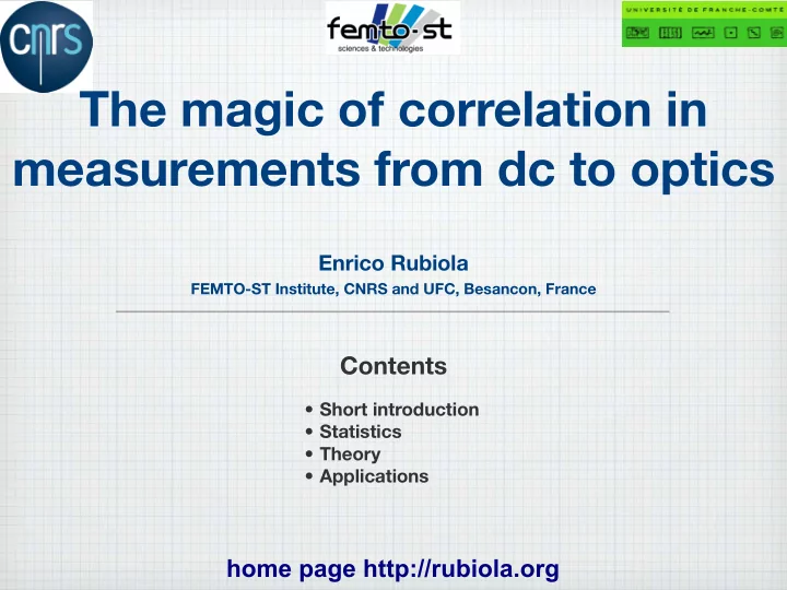
The magic of correlation in measurements from dc to optics Enrico - PowerPoint PPT Presentation
The magic of correlation in measurements from dc to optics Enrico Rubiola FEMTO-ST Institute, CNRS and UFC, Besancon, France Contents Short introduction Statistics Theory Applications home page http://rubiola.org 2
The magic of correlation in measurements from dc to optics Enrico Rubiola FEMTO-ST Institute, CNRS and UFC, Besancon, France Contents • Short introduction • Statistics • Theory • Applications home page http://rubiola.org
2 Correlation measurements x = a + c instrument A Σ a ( t ) FFT analyzer dual-channel instr. noise c ( t ) DUT input y = b + c instrument B signal Σ b ( t ) instr. noise Two separate instruments a(t), b(t) –> instrument noise measure the same DUT. c(t) –> DUT noise Only the DUT noise is common noise measurements single-channel DUT noise, a, b instrument noise S � (f) normal use c DUT noise background, a, b instrument noise 1/ � m ideal case c = 0 no DUT c is the correlated background, a, b correlation instrument noise real case c ≠ 0 Zero DUT noise frequency
3 Boring exercises before playing a Steinway
4 Fourier Statistics
5 Vocabulary of statistics • A random process x(t) is defined through a random experiment e that associates a function x e (t) with each outcome e . • The set of all the possible x e (t) is called ensemble • The function x e (t) is called realization or sample function . • The ensemble average is called mathematical expectation E { } • A random process is said stationary if its statistical properties are independent of time. • Often we restrict the attention to some statistical properties. • In physics, this is the concept of repeatability. • A random process x(t) said ergodic if a realization observed in time has the statistical properties of the ensemble. • Ergodicity makes sense only for stationary processes. • Often we restrict the attention to some statistical properties. • In physics, this is the concept of reproducibility. Example: thermal noise of a resistor of value R • The experiment e is the random choice of a resistor e • The realization x e (t) is the noise waveform measured across the resistor e • We always measure <x 2 >=4kTRB, so the process is stationary • After measuring many resistors, we conclude that <x 2 >=4kTRB holds always. The process is ergodic.
6 Formal definition of the PSD for stationary random process x(t) Autocovariance � � C ( τ ) = E [x( t + τ ) − µ ][x ∗ ( t ) − µ ] Improperly referred to as the correlation and denoted with R xx ( τ ) � � µ = E x � ∞ PSD (two-sided) � � S ( ω ) = F C ( τ ) = C ( τ ) e − ı ωτ d τ In mathematics, called spectral measure −∞ � T/ 2 For stationary ergodic process, interchange C ( τ ) = lim [ x ( t + τ ) − µ ][ x ∗ ( t ) − µ ] dt ensemble and time average T →∞ − T/ 2 process x( t ) –> realization x ( t ) 1 1 T | X T ( ω ) | 2 S ( ω ) = lim T X T ( ω ) X ∗ T ( ω ) = lim Wiener Khinchin theorem T →∞ T →∞ for stationary ergodic processes S I ( f ) = 2 S II ( ω / 2 π ) , f > 0 In experiments we use the single-sided PSD Fourier transform autocorrelation function � ∞ R xx ( τ ) = 1 � � � � ξ ( t ) e − ı ω t dt = [x( t ) − µ ][x( t − τ ) − µ ] F ξ σ 2 E −∞
7 A relevant property of random noise A theorem states that there is no a-priori relation between PDF and spectrum For example, white noise can originate from • Poisson process (emission of a particle at random time) • Random telegraph (random switch between two level) • Thermal noise (Gaussian) PDF = Probability Density Function
8 Sum of random variables 1. The sum of Gaussian distributed random variables has Gaussian PDF 2. The central limit theorem states that For large m , the PDF of the the sum of m statistically independent processes tends to a Gaussian distribution Let X = X 1 +X 2 +…+X m be the sum of m processes of mean µ 1 , µ 2 , … µ m and variance σ 12 , σ 22 , … σ m2 . The process X has Gaussian PDF expectation E{X} = µ 1 + µ 2 +…+ µ m , and variance σ 2 = σ 12 + σ 22 +…+ σ m2 3. Similarly, the average <X> m = (X 1 +X 2 +…+X m )/m has Gaussian PDF, E{X} = ( µ 1 + µ 2 +…+ µ m )/m, and σ 2 = ( σ 12 + σ 22 +…+ σ m2 )/m 4. Since white noise and flicker noise arise from the sum of a large number of small-scale phenomena, they are Gaussian distributed PDF = Probability Density Function
9 Product of independent zero-mean Gaussian-distributed random variables x 1 and x 2 are normal distributed with f ( x ) = 1 � − | x | � πσ K 0 zero mean and variance σ 12 , σ 22 σ x = x 1 x 2 E { f ( x ) } = 0 x has Bessel K 0 distribution E {| f ( x ) − E { f ( x ) }| 2 } = σ 2 with variance σ = σ 12 σ 22 Thanks to the central limit theorem, the average <X> m = (X 1 +X 2 +…+X m )/m of m products has • Gaussian PDF, • average E{X} = 0 • variance V{X} = σ 2
10 Properties of white Gaussian noise with zero mean x(t) <=> X(f) = X’(f)+ ıX”(f) 1. Central limit theorem: x(t) <=> X(f) are Gaussian distributed 2. Energy equipartition (frequency): 1. X(f 1 ) and X(f 2 ), f 1 ≠ f 2 , are statistically independent, 2. var{X(f 1 )} = var{X(f 2 )} statistically independent 3. Energy equipartition (Re-Im): X' 1. X’ and X” are statistically statistically f 0 f 1 f N–1 /2 independent f 2 independent 2. var{X’} = var{X”} = var{X}/2 X" 4. Sum: Y = X 1 + X 2 statistically independent 1. Y is Gaussian distributed 2. var{Y} = var{X 1 } + var{X 2 } 5. Product: Y = X 1 × X 2 a real process has 1. Y has distribution Bessel K 0 (|y|) / π N degrees of freedom 2. var{Y} = var{X 1 } × var{X 2 }
11 Properties of flicker noise (Gaussian distributed, with zero mean) x(t) <=> X(f) = X’(f)+ ıX”(f) 1. Central limit theorem: x(t) and X(f) end up to be Gaussian statistically independent 2. Power distribution (frequency) 1. X(f 1 ) and X(f 2 ), f 1 ≠ f 2 , are statistically X' independent f 0 f 1 can be f N–1 /2 f 2 2. var{X(f 2 )} < var{X(f 1 )} for f 2 > f 1 correlated X" 3. Real and imaginary part 1. X’ and X” can be correlated statistically independent 2. var{X’} ≠ var{X”} ≠ var{X}/2 4. Y = X 1 + X 2 , zero-mean Gaussian r.v. Central limit theorem: var{Y} = var{X 1 } + var{X 2 } x(t) and X(f) end up to be Gaussian 5. If X 1 and X 2 are zero-mean Gaussian r.v., the product Y = X 1 × X 2 , 1. has distribution Bessel K0(|y|) / π 2. has var{Y} = var{X 1 } var{X 2 }
12 Statistics & finite-duration measurement x(t) X(f) product convolution T sinc( π Tf) Π (t/T) T 1 t f –T/2 +T/2 1/4T result result x T (t) X T (f) x(t) Π (t/T) X(f) * T sinc( π Tf) File: xsp-truncation-effect • The convolution with sinc( ) scrambles the spectrum, spreading the power of a single point all around. This introduces correlation • In the presence of large peaks or sharp roll-off, this is disturbing • In the measurement of smooth noise, often negligible • Further consequences in cross-correlation measurements
13 Normal (Gaussian) distribution − ( x − µ ) 2 1 � � x is normal distributed with f ( x ) = 2 π σ exp √ 2 σ 2 zero mean μ and variance σ 2 E { f ( x ) } = µ E { f 2 ( x ) } = µ 2 + σ 2 E {| f ( x ) − E { f ( x ) }| 2 } = σ 2 − ( x − µ ) 2 � � 1 f ( x ) = 2 π σ exp √ 2 σ 2 � � P N = P { x < 0 } = 1 µ � � P P = P { x > 0 } = 1 − 1 µ 2erfc σ σ 2erfc √ √ 2 σ 2 σ x < 0 x > 0 File: xsp-Gaussian 0 µ x µ + σ µ − σ 1 1 σ σ µ N = µ − µ P = µ + � � � � � � 2 π exp( µ 2 / σ 2 ) 2 π exp( µ 2 / σ 2 ) µ µ 1 1 − 1 2 erfc 2 erfc √ √ 2 σ 2 σ
14 One-sided Gaussian distribution x is normal distributed with − x 2 � � 1 f ( x ) = 2 2 π σ exp zero mean and variance σ 2 √ 2 σ 2 � 2 y = | x | E { f ( x ) } = π σ E { f 2 ( x ) } = σ 2 � � 1 − 2 E {| f ( x ) − E { f ( x ) }| 2 } = σ 2 π one-sided Gaussian distribution with σ 2 = 1 / 2 quantity value with σ 2 = 1 / 2 [10 log( ), dB] $"' � 1 -./ ! !"0/0&#%1!!"%.&0"!23"412"5. 0.564 $"& average = [ − 2 . 49] $"% π $"$ � 1 2 − 1 0.426 deviation = $"! !"#$%&'&()*+ [ − 3 . 70] π !"+ !"* � π dev 0.756 avg = 2 − 1 !") [ − 1 . 22] !"( !"#$%&'&+ � !"# avg + dev 1 2 − 1 1.756 = 1 + !"' [+2 . 44] avg π !"& !"#$%&'&+),+ � avg − dev 1 2 − 1 0.244 !"% = 1 − !"$ [ − 6 . 12] avg ,-./012/ ! 3-4/4 ! 56733 ! 4-389-: π ;"0<7:-1.6=0>?90%!!* !"! !"! !"# $"! $"# %"! %"# &"! &"# '"! '"# #"! � avg + dev 7.18 avg − dev = 1 + 1 / 2 − 1 / π � [8 . 56] 1 − 1 / 2 − 1 / π
15 Chi-square distribution x i are normal distributed with Notice that the sum of zero mean and equal variance σ 2 χ 2 is a χ 2 distribution r � m m χ 2 = x 2 � � χ 2 = χ 2 i j , r = r j i =1 j =1 j =1 is χ 2 distributed with r degrees of freedom !') )*+ ! ,-./!0 2 − 1 e − x 2 r f ( x ) = x 2 !"#"$ x ≥ 0 !'# � 1 � r 2 Γ 2 r 2 !'( E { f ( x ) } = σ 2 r !"#"% !'" E { [ f ( x )] 2 } = σ 4 r ( r + 2) !"#"& !"#"' !'& !"#"$( E {| f ( x ) − E { f ( x ) }| 2 } = 2 σ 4 r *+,-./0+ ! 12345- ! 6+175+8 9'.:38+;,4<.=>5."!!% !'! ! " # $ % &! &" &# &$ &% "! z ! = Γ ( z + 1) , z ∈ N
Recommend
More recommend
Explore More Topics
Stay informed with curated content and fresh updates.
