The Fractional Poisson: a Simple Dose-Response Model Mike Messner - PowerPoint PPT Presentation
The Fractional Poisson: a Simple Dose-Response Model Mike Messner U. S. EPA Office of Water Messner.Michael@epa.gov Image of Norovirus from RCSB Outline Single-hit theory & models for microbial dose- response Norovirus & the
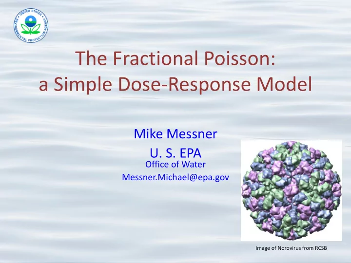
The Fractional Poisson: a Simple Dose-Response Model Mike Messner U. S. EPA Office of Water Messner.Michael@epa.gov Image of Norovirus from RCSB
Outline • Single-hit theory & models for microbial dose- response • Norovirus & the beta-Poisson model • The fractional Poisson model • Other candidates for fractional Poisson • What’s next?
Single-hit Theory • A volunteer agrees to ingest a capsule containing a “known amount” of some microbial pathogen (could be virus, bacteria, protozoa, other “bugs”) • The individual pathogen is “successful” if it overcomes any barriers and is able to initiate an infection in the host. As a result of the infection, lots and lots of newly-minted bugs are created and released to keep things going well for the bug (an poorly for the host). • The single-hit idea is that, when any one bug is successful, the host is infected and what happens to the other bugs is not important. It only takes one. • The host can’t be infected unless at least one bug is ingested.
Single-hit Models • Two popular single-hit models: – Exponential – Beta-Poisson • Exponential – Dose is Poisson. – Each bug succeeds with probability P, and independently of other bugs. • Beta-Poisson – Same as exponential, but P varies from host-to-host as a beta random variable
Human Challenge Studies • A series of human challenge studies have been conducted to identify norovirus infectivity. • Human subjects ingest volumetrically-prepared doses. – Assumption: Particles are randomly dispersed, so actual number ingested is a Poisson random variable – Viruses were either aggregated (particle is many virions stuck together) or disaggregated (particle is single virion) • Norovirus only binds to epithelial cells of subjects with positive ABH antigen secretor status (Se+). Se- subjects appear to be well- protected against infection. – Se- individuals do not possess a gene associated with a norovirus binding receptor. – We focus on Se+ subjects. – About 80% of people are Se+.
Beta Distribution Two parameters (usually a and b ) • • Defined between 0 and 1 (exclusive: 0 and 1 are excluded) Density function, dbeta(r, a,b ) , can have different shapes • – Normal when a and b are large – Lognormal when a is small and b not – Bathtub when a and b are both small • Describes variation in host susceptibility Converges to exponential as a and b become huge • As a and b become tiny, the probability mass is squeezed to 0 and • 1. – 0 and 1 are really important. – But 0 and 1 are excluded. – Maybe some other model is needed.
Various Shapes for Beta-Poisson 4 alpha = 1, beta = 1 alpha = 0.5, beta = 0.5 alpha = 5, beta = 1 alpha = 1, beta = 3 alpha = 2, beta = 2 3 alpha = 2, beta = 5 alpha = 5, beta = 5 Probability Density 2 1 0 0.0 0.2 0.4 0.6 0.8 1.0 x
Estimates are Based on Data • Data from human challenge studies • Se- subjects are immune, so we focus on the Se+ subjects. The virus is able to bind on cell surfaces and reproduce in only these subjects. • At a particular dose, number infected is binomial random variable with parameters: n = number subjects and p = Pr{infection|dose, a, b } • Data includes k = the number infected (of the n subjects)
Beta-Poisson Infection Probability & Likelihood • p = Pr{infection|dose, a, b } is given by • Number infected is k with probability (a.k.a. “likelihood”) = dbinom(k, n, p)
Data • Four studies: – Teunis et al . 2008 (beta-Poisson model, 11 dose groups, some disaggregated) – Seitz et al. 2011 (1 disaggregated dose group) – Frenck et al. 2012 (1 aggregated dose groups) – Atmar et al. 2013 (4 aggregated dose group) • A dose group is a set of subjects, each dosed at the same level (measured as genomic equivalent copies)
Dose Inoculum Total Subjects Infected R5ef Subjects 3.24 Aggregated 8 0 Teunis Aggregated 32.4 9 0 Teunis 324 Aggregated 9 3 Teunis 3240 Aggregated 3 2 Teunis Aggregated 324,000 8 7 Teunis 3.24 * 10 6 Aggregated 7 3 Teunis 3.24 * 10 7 Aggregated 3 2 Teunis 3.24 * 10 8 Aggregated 6 5 Teunis 6.92 * 10 5 Disaggregated 8 3 Teunis 6.92 * 10 6 Disaggregated 18 14 Teunis 6.92 * 10 7 Disaggregated 1 1 Teunis 6.5 * 10 7 Disaggregated 13 10 Seitz 192 Aggregated 13 1 Atmar Aggregated 1920 13 7 Atmar 19,200 Aggregated 8 7 Atmar 1.92 * 10 6 Aggregated 7 6 Atmar 2 * 10 7 Aggregated 23 16 Frenck
Estimating a and b • Bayesian, using noninformative priors • Account for aggregation in some inocula • To avoid numerical issues, use confluent hypergeometric functions with R-Code provided by Dr. Peter Teunis • Markov Chain Monte Carlo sample of parameters a, b, and m (aggregation parm)
Where we came in! • Try to reproduce Peter Teunis’ 2008 estimate. – Based on 11 dose groups (1 st 11 rows of our table) • Not easy! – Some data in paper had 10x error. – Confluent hypergeometric function took some effort to check (R and MathCAD) • Success! – Got same max likelihood parameter estimates. a = 0.040 b = 0.055 mean aggregate size = 396.
But • Likelihood contours and MCMC sample had “issues” – MCMC sample of size 10K had about 1.3K unique values (suggests poor mixing) – MCMC sample thinned where it shouldn’t (influence of normal prior) – Parameters a and b were small. (Probability mass is concentrated near 0 and 1.)
The MCMC Sample
The Max Likelihood Beta Density
It gets even more extreme.
So…the beta - Poisson doesn’t work well for Norovirus. • MCMC sample thinned- out, but shouldn’t have with a truly non-informative prior. • Bathtub is extremely deep. – Only 27% of the mass is shown in the figure! – 73% of the probability mass falls below 0.001 or above 0.999. – More than 1/3 of the probability mass falls below 0.000001 (1/million). – Another large fraction falls above 0.999999. Most subjects are almost perfectly susceptible or almost perfectly immune to infection. Why not exclude everything BUT 0 and 1? (Subjects would be either perfectly susceptible or perfectly immune.)
Fractional Poisson • If we exclude everything but 0 and 1: • Each Se+ subject is either perfectly susceptible or perfectly immune. • Let P = fraction perfectly susceptible (parameter is 0) • 1 – P = fraction perfectly immune (parameter is 1) • Perfectly susceptible subjects are infected if and only if they ingest at least one norovirus or norovirus aggregate.
Fractional Poisson is simple! • Fraction P perfectly susceptible • Poisson dose (with mean l ) – If large, probability of ingesting zero is nil. – If not large, probability of ingesting zero is Poisson probability of zero: e - l – Probability of ingesting one or more = 1 - e - l • Aggregation – Probability of ingesting zero = e -l/m – Probability of ingesting one or more = 1 - e - l/m – Need to estimate mean aggregate size ( m ). – Aggregate size distribution is not important.
Estimating P and m was simple! • We found max likelihood solution: P = 0.722 and mean aggregate size is 987 • Likelihood is almost the same as for the beta-Poisson. • AIC* favors fractional Poisson over beta-Poisson • Likelihood contours and MCMC sample agree. • Error structure is nearly normal. • Estimation error is small (compared to beta- Poisson) * AIC = Akaike Information Criterion
Code for Infection Probability (disaggregated dose) Beta-Poisson Fractional Poisson drbp<-function(alpha,beta,dose) 1-(1+dose/beta)^(-alpha) P * (1-exp(-dose)) dr1f1 <- function(alpha,beta,dose) { if(dose<1E-4) return (alpha*dose/(alpha+beta)) # Corrected if(alpha>1E3 && beta < alpha/100) return (1-exp(-dose)) if(alpha>1E2 && beta>1E5) return (1-exp(-dose*alpha/beta)) if(alpha>1E1 && beta>1E5 && dose*alpha/beta>10) return (drbp(alpha,beta,dose)) if(alpha>1 && beta>alpha*20 && dose>10) return (drbp(alpha,beta,dose)) if(alpha>1 && beta>alpha && dose>50) return (drbp(alpha,beta,dose)) if(alpha>1 && beta<alpha && dose>20) return (drbp(alpha,beta,dose)) if(alpha<1 && beta>alpha*50) return (drbp(alpha,beta,dose)) if(alpha<0.1 && beta>alpha*20) return (drbp(alpha,beta,dose)) if(abs(round(alpha)-alpha)<1E-4) alpha=1.0001*alpha if(abs(round(beta)-beta)<1E-4) beta=1.0001*beta return (1-hyperg_1F1(alpha,alpha+beta,-dose)) }
Normal contours. Well-behaved MCMC sample.
Estimated Infection Probability Beta-Poisson Fractional Poisson
95% prediction intervals at Dose == 1 • Beta-Poisson: 0.019 to 0.76 • Fractional Poisson: 0.63 to 0.8 But: We haven’t ruled out the beta model. We really have no low dose data, so we wouldn’t be surprised if new low dose data were to favor the beta model.
Imagine a new study… What if 10 Se+ individuals each ingested exactly 1 virion and none was infected? That would not be likely under the fractional model. Likelihood would favor the beta. If instead , 5 to 10 were infected, that would be consistent with both models. Again, the fractional Poisson would be the model of choice, due to having fewer parameters.
Recommend
More recommend
Explore More Topics
Stay informed with curated content and fresh updates.
