The Folklore Theorem Return to the general mean-variance - PowerPoint PPT Presentation

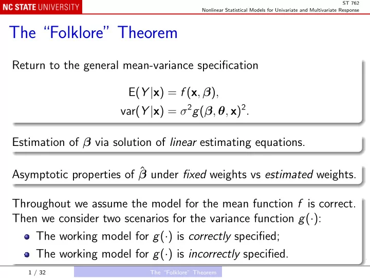
ST 762 Nonlinear Statistical Models for Univariate and Multivariate Response The “Folklore” Theorem Return to the general mean-variance specification E( Y | x ) = f ( x , β ) , var( Y | x ) = σ 2 g ( β , θ , x ) 2 . Estimation of β via solution of linear estimating equations. Asymptotic properties of ˆ β under fixed weights vs estimated weights. Throughout we assume the model for the mean function f is correct. Then we consider two scenarios for the variance function g ( · ): The working model for g ( · ) is correctly specified; The working model for g ( · ) is incorrectly specified. 1 / 32 The “Folklore” Theorem

ST 762 Nonlinear Statistical Models for Univariate and Multivariate Response Iterative GLS scheme ∗ and ˆ Preliminary estimators ˆ θ . β σ and ˆ Update ˆ θ by solving ∗ �� 2   � � x j , ˆ Y j − f n β ∗ , ˆ � � � ˆ − 1  τ θ β θ , x j = 0 ,   � 2  � ∗ , ˆ ˆ σ 2 g ˆ θ , x j β j =1 where � � 1 τ θ ( β , θ , x ) = . ν θ ( β , θ , x ) 2 / 32 The “Folklore” Theorem

ST 762 Nonlinear Statistical Models for Univariate and Multivariate Response Then update ˆ β by solving � � x j , ˆ Y j − f n β � � � x j , ˆ � 2 × f β β = 0 . ∗ , ˆ � ˆ θ , x j g β j =1 ∗ in this update. Note that the β argument of g ( · ) is held at ˆ β Iterate the last two steps C times, possibly to convergence ( C = ∞ ). 3 / 32 The “Folklore” Theorem

ST 762 Nonlinear Statistical Models for Univariate and Multivariate Response The theorem Suppose that √ n ∗ − β 0 � � ˆ = O p (1) β and √ n � � ˆ θ − θ 0 = O p (1) θ are √ n -consistent). ∗ and ˆ (i.e., ˆ β Then, under suitable regularity conditions, √ n � � ˆ L 0 , σ 2 � � β − β 0 − → N . 0 Σ WLS 4 / 32 The “Folklore” Theorem

ST 762 Nonlinear Statistical Models for Univariate and Multivariate Response Here � − 1 � n →∞ n − 1 X T WX Σ WLS = lim where f β ( x 1 , β 0 ) T   f β ( x 2 , β 0 ) T   X = X ( β 0 ) =  ,  .  .   .  f β ( x n , β 0 ) T W = diag( w 1 , w 2 , . . . , w n ) , 1 w j = g ( β 0 , θ 0 , x j ) 2 . 5 / 32 The “Folklore” Theorem

ST 762 Nonlinear Statistical Models for Univariate and Multivariate Response Derivation n � − 2 � � � �� � � 0 = n − 1 / 2 � ˆ ∗ , ˆ x j , ˆ x j , ˆ g β θ , x j Y j − f β f β β j =1 n ≈ n − 1 / 2 � g ( β 0 , θ 0 , x j ) − 2 { Y j − f ( x j , β 0 ) } f β ( x j , β 0 ) j =1  n  n − 1 � + { Y j − f ( x j , β 0 ) } f ββ ( x j , β 0 ) j =1  n  n 1 / 2 � � ˆ − n − 1 � g ( β 0 , θ 0 , x j ) − 2 f β ( x j , β 0 ) f β ( x j , β 0 ) T β − β 0 j =1   n ∗ − β 0  n 1 / 2 � �  − 2 n − 1 � g ( β 0 , θ 0 , x j ) − 3 { Y j − f ( x j , β 0 ) } f β ( x j , β 0 ) g β ( β 0 , θ 0 , x j ) T ˆ + β j =1   n  n 1 / 2 � �  − 2 n − 1 � g ( β 0 , θ 0 , x j ) − 3 { Y j − f ( x j , β 0 ) } f β ( x j , β 0 ) g θ ( β 0 , θ 0 , x j ) T ˆ + θ − θ 0 j =1 6 / 32 The “Folklore” Theorem

ST 762 Nonlinear Statistical Models for Univariate and Multivariate Response Rewrite as: ∗ − β 0 )+ E n n 1 / 2 (ˆ 0 ≈ C n +( A n 1 + A n 2 ) n 1 / 2 (ˆ β − β 0 )+ D n n 1 / 2 (ˆ θ − θ 0 ) β where n w 1 / 2 C n = σ 0 n − 1 / 2 � f β ( x j , β 0 ) ǫ j j j =1 n � w 1 / 2 A n 1 = σ 0 n − 1 f ββ ( x j , β 0 ) ǫ j j j =1 n A n 2 = − n − 1 � w j f β ( x j , β 0 ) f β ( x j , β 0 ) T j =1 n w j f β ( x j , β 0 ) ν β ( β 0 θ 0 x j , ) T ǫ j D n = − 2 σ 0 n − 1 � j =1 n w j f β ( x j , β 0 ) ν θ ( β 0 θ 0 x j , ) T ǫ j E n = − 2 σ 0 n − 1 � j =1 7 / 32 The “Folklore” Theorem

ST 762 Nonlinear Statistical Models for Univariate and Multivariate Response Also ǫ j = Y j − f ( x j , β 0 ) σ 0 g ( β 0 , θ 0 , x j ) so that E ( ǫ j | x j ) = 0 and var( ǫ j | x j ) = 1 . 8 / 32 The “Folklore” Theorem

ST 762 Nonlinear Statistical Models for Univariate and Multivariate Response We have that p − → 0 A n 1 p → − Σ − 1 − A n 2 WLS L 0 , σ 2 0 Σ − 1 � � − → N C n WLS p D n − → 0 p E n − → 0 so p → − Σ − 1 A n = A n 1 + A n 2 − WLS 9 / 32 The “Folklore” Theorem

ST 762 Nonlinear Statistical Models for Univariate and Multivariate Response Then √ n � � ˆ ≈ − A − 1 β − β 0 n C n L 0 , σ 2 � � − → N 0 Σ WLS , as claimed. 10 / 32 The “Folklore” Theorem

ST 762 Nonlinear Statistical Models for Univariate and Multivariate Response Remarks This is the same large-sample distribution as for the WLS estimator with known weights. That is, to this order of approximation, using estimated weights gives the same sampling distribution as if the weights were known. ∗ and ˆ The terms D n and E n corresponding to the “effects” of ˆ θ , β respectively, are o p (1). This implies that the estimators we substitute for β and θ in the weights play no role in determining the large sample properties of the resulting estimator ˆ β . Because the effect of ˆ θ is also negligible, as E n = o p (1), it implies that how one estimates θ does not matter in determining the properties of the resulting GLS estimator. 11 / 32 The “Folklore” Theorem

ST 762 Nonlinear Statistical Models for Univariate and Multivariate Response The main “folklore” message The large sample precision is unaffected not only by the need to estimate the parameters in the weights, but how these parameters are estimated, as long as they are estimated “sensibly.” The result is true for any C : C = 1 for a one-step estimator, C = ∞ for a converged iterated estimator. Here we have assumed that the variance function g ( · ) is correctly specified. 12 / 32 The “Folklore” Theorem

ST 762 Nonlinear Statistical Models for Univariate and Multivariate Response The folklore result implies that � � − 1 � � X ( β 0 ) T W ( β 0 , θ 0 ) X ( β 0 ) · ˆ β 0 , σ 2 ∼ N . β 0 We use this by plugging in ˆ β , ˆ θ , and �� 2 � � x j , ˆ n Y j − f β 1 σ 2 = � ˆ . � 2 n − p � β , ˆ ˆ g θ , x j j =1 This is the approximation used by SAS’s proc nlin and the R function nls . 13 / 32 The “Folklore” Theorem

ST 762 Nonlinear Statistical Models for Univariate and Multivariate Response Working Variances Recall the general mean-variance specification E( Y | x ) = f ( x , β ) , var( Y | x ) = σ 2 g ( β , θ , x ) 2 . Suppose we use the GLS scheme with the correct mean specification, but a working variance specification var( Y | x ) = τ 2 h ( β , γ , x ) 2 . τ 2 and ˆ γ estimate, and what is the consequence for ˆ What do ˆ β ? 14 / 32 The “Folklore” Theorem

ST 762 Nonlinear Statistical Models for Univariate and Multivariate Response We solve ∗ �� 2 � 2   � � � ∗ , ˆ x j , ˆ ˆ τ 2 h Y j − f β − ˆ β γ , x j n � ∗ , ˆ � � ˆ  ξ γ γ , x j = 0 , β   � 2  � ∗ , ˆ ˆ h β γ , x j j =1 where � 1 � ξ γ ( β , γ , x ) = . ∂ log h ( β , γ , x ) ∂ γ Suppose that there exist γ n and τ 2 n such that { Y j − f ( x j , β ) } 2 − τ 2 � n � � � n h ( β , γ n , x j ) 2 � E ξ γ ( β , γ n , x j ) = 0 . h ( β , γ n , x j ) 2 j =1 15 / 32 The “Folklore” Theorem

ST 762 Nonlinear Statistical Models for Univariate and Multivariate Response τ 2 as estimators of γ n and τ 2 Then we can view ˆ γ and ˆ n . Also, if γ n → γ ∗ and τ 2 n → τ ∗ 2 , then (consistency): p p → τ ∗ 2 . → γ ∗ τ 2 γ ˆ − and ˆ − More strongly ( √ n -consistency): √ n (ˆ √ n τ 2 − τ ∗ 2 � γ − γ ∗ ) = O p (1) � and ˆ = O p (1) . Note In general, if we fit a parametric model f ( x , θ ) to data from another density f 0 ( x ), the MLE estimates the parameter values θ ∗ that minimize the Kullback-Leibler distance from f 0 ( · ) to f ( · , θ ). 16 / 32 The “Folklore” Theorem

ST 762 Nonlinear Statistical Models for Univariate and Multivariate Response Asymptotic distribution of ˆ β Using similar methods to those used earlier, we show that � � − 1 � � − 1 � ˆ · β 0 , σ 2 � X T UX X T UW − 1 UX � � X T UX ∼ N . β 0 17 / 32 The “Folklore” Theorem

ST 762 Nonlinear Statistical Models for Univariate and Multivariate Response Here, as before,  f β ( x 1 , β 0 ) T  f β ( x 2 , β 0 ) T   X = X ( β 0 ) =  ,  .  .   .  f β ( x n , β 0 ) T W = diag( w 1 , w 2 , . . . , w n ) , 1 w j = g ( β 0 , θ 0 , x j ) 2 , U = diag( u 1 , u 2 , . . . , u n ) , 1 u j = h ( β 0 , γ ∗ , x j ) 2 . 18 / 32 The “Folklore” Theorem

ST 762 Nonlinear Statistical Models for Univariate and Multivariate Response Notes Note that this is the same asymptotic distribution as in the fixed working weights case. The original “folklore” theorem is the special case where the working variance function h ( · ) is the same as the true variance function g ( · ). The efficiency discussion carries over immediately from the fixed weights case. 19 / 32 The “Folklore” Theorem