The Evolution of Cosmological Perturbations in F(R)-gravity Sante - PowerPoint PPT Presentation

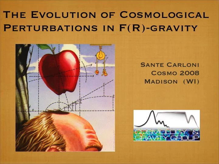
The Evolution of Cosmological Perturbations in F(R)-gravity Sante Carloni Cosmo 2008 Madison (WI)

Dark Energy (DE ) In the last few years the traditional picture of the cosmos has changed completely

Dark Energy (DE ) In the last few years the traditional picture of the cosmos has changed completely

Dark Energy (DE ) In the last few years the traditional picture of the cosmos has changed completely +

Dark Energy (DE ) In the last few years the traditional picture of the cosmos has changed completely +

Dark Energy (DE ) In the last few years the traditional picture of the cosmos has changed completely + Many different models for dark energy have been proposed so far. We will focus on the ones based on Fourth Order Gravity (FOG)

Fourth Order Gravity In homogeneous and isotropic spacetimes a general action for fourth order gravity in presence of matter is � � d 4 x √− g f ( R ) + d 4 x √− g L M . A =

Fourth Order Gravity In homogeneous and isotropic spacetimes a general action for fourth order gravity in presence of matter is � � d 4 x √− g f ( R ) + d 4 x √− g L M . A = varying with respect to the metric gives f ′ ( R ) R ab − 1 2 f ( R ) g ab = f ′ ( R ) ; cd ( g ca g db − g cd g ab ) + ˜ T M ab , where δ ( √− gL M ) 2 ˜ T M ab = √− g δ g ab and the “prime” denotes the derivative with respect to the Ricci scalar.

DE and FOG Why Fourth order gravity is an interesting model for DE?

DE and FOG Why Fourth order gravity is an interesting model for DE? Differently from GR, they admit naturally cosmological solutions characterized by accelerated expansion i.e. the footprint of DE They are recovered as low energy limit of more fundamental schemes like M-theory, supergravity etc.

DE and FOG Why Fourth order gravity is an interesting model for DE? Differently from GR, they admit naturally cosmological solutions characterized by accelerated expansion i.e. the footprint of DE They are recovered as low energy limit of more fundamental schemes like M-theory, supergravity etc. Unfortunately, due to their high degree of non linearity, this kind of theories are particularly difficult to deal with.

DE and FOG Why Fourth order gravity is an interesting model for DE? Differently from GR, they admit naturally cosmological solutions characterized by accelerated expansion i.e. the footprint of DE They are recovered as low energy limit of more fundamental schemes like M-theory, supergravity etc. Unfortunately, due to their high degree of non linearity, this kind of theories are particularly difficult to deal with. So one needs to develop new techniques to be able to unfold their properties

1+3 covariant approach Given the vector field associated to a time-like flow in the model:

1+3 covariant approach Given the vector field associated to a time-like flow in the model: Bianchi Identities Ricci Identities

1+3 covariant approach Given the vector field associated to a time-like flow in the model: 1+3 Equations Bianchi Identities u a , ω ab , µ i , p i ) ( Θ , σ ab , ˙ Ricci Identities

1+3 covariant approach Given the vector field associated to a time-like flow in the model: 1+3 Equations Bianchi Identities u a , ω ab , µ i , p i ) ( Θ , σ ab , ˙ Ricci Identities equivalent to the einstein eqns

1+3 covariant approach Given the vector field associated to a time-like flow in the model: 1+3 Equations Bianchi Identities u a , ω ab , µ i , p i ) ( Θ , σ ab , ˙ Ricci Identities equivalent to the einstein This approach has many advantages: eqns its variables have a clear physical meaning at any stage of the calculations and are gauge invariant the treatment of both the exact and the linearized theory is considerably simplified the same variables can be used in perturbing different models e.g anisotropic spacetimes etc. it is easily adaptable to alternative gravity

Scalar Perturbation variables

Scalar Perturbation variables The natural set of inhomogeneity variables associated with the spherical collapse in GR are: ∆ m = S 2 ˜ ∇ 2 µ Z = S 2 ˜ C = S 4 ˜ ∇ 2 ˜ ∇ 2 Θ R µ

Scalar Perturbation variables The natural set of inhomogeneity variables associated with the spherical collapse in GR are: ∆ m = S 2 ˜ ∇ 2 µ Z = S 2 ˜ C = S 4 ˜ ∇ 2 ˜ ∇ 2 Θ R µ Matter fluctuations

Scalar Perturbation variables The natural set of inhomogeneity variables associated with the spherical collapse in GR are: ∆ m = S 2 ˜ ∇ 2 µ Z = S 2 ˜ C = S 4 ˜ ∇ 2 ˜ ∇ 2 Θ R µ Matter fluctuations Expansion fluctuations (related to the first derivative of μ )

Scalar Perturbation variables The natural set of inhomogeneity variables associated with the spherical collapse in GR are: ∆ m = S 2 ˜ ∇ 2 µ Z = S 2 ˜ C = S 4 ˜ ∇ 2 ˜ ∇ 2 Θ R µ Matter fluctuations Expansion fluctuations 3-Ricci scalar fluctuations (related to the first derivative of μ )

Scalar Perturbation variables The natural set of inhomogeneity variables associated with the spherical collapse in GR are: ∆ m = S 2 ˜ ∇ 2 µ Z = S 2 ˜ C = S 4 ˜ ∇ 2 ˜ ∇ 2 Θ R µ Matter fluctuations Expansion fluctuations 3-Ricci scalar fluctuations (related to the first derivative of μ ) together with: R = S 2 ˜ ℜ = S 2 ˜ ∇ 2 ˙ ∇ 2 R R Ricci “momentum” Ricci Scalar fluctuation fluctuations

Scalar Perturbation variables The natural set of inhomogeneity variables associated with the spherical collapse in GR are: ∆ m = S 2 ˜ ∇ 2 µ Z = S 2 ˜ C = S 4 ˜ ∇ 2 ˜ ∇ 2 Θ R µ Matter fluctuations Expansion fluctuations 3-Ricci scalar fluctuations (related to the first derivative of μ ) together with: R = S 2 ˜ ℜ = S 2 ˜ ∇ 2 ˙ ∇ 2 R R Ricci “momentum” Ricci Scalar fluctuation fluctuations

Perturbation equations

Perturbation equations We can then derive the evolution equations for these variables. Using the covariant harmonics defined by ∇ 2 Q = − k 2 ˜ S 2 Q ,

Perturbation equations We can then derive the evolution equations for these variables. Using the covariant harmonics defined by ∇ 2 Q = − k 2 ˜ S 2 Q , we obtain �� 2 � � � ˙ S 2 − w (3 p R + µ R ) − 2 w ˙ 3 w 2 − 1 w k 2 � � � µ Rf ′′ R Θ f ′′ ¨ ˙ ∆ ( k ) ∆ ( k ) ∆ ( k ) m + Θ − 3 − w m − − m f ′ f ′ f ′ R Θ f ′′ � f ′′ 2 k 2 R Θ f (3) = 1 � � R ( k ) − ( w + 1) Θ f ′′ � R ( k ) , f − 2 µ + 2 ˙ f ′ 2 − 2 ˙ ˙ S 2 f ′′ − 1 + 2( w + 1) f ′ f ′ � k 2 S 2 f ′′ + 2 2 f ′ f ′′ − 1 S 2 f ′′ + 2 K 9 Θ 2 f ′′ − ( w + 1) µ f ′′ ¨ R ( k ) + � Θ f ′′ + 2 ˙ Rf (3) � 6( µ R + 3 p R ) f ′′ ˙ R ( k ) − R Θ f ′′ 2 � � 1 − f ′ 3 + f 6 f ′ f ′′ + ˙ Rf (3) − Θ f (3) ˙ R − f (4) ˙ R ( k ) = − 6 f ′ − ¨ R 2 3(3 w − 1) µ m − ( w − 1) ˙ Rf ′′ �� Rf ′′ w � f (3) ˙ R 2 + ( p R + µ R ) f ′ + 7 R Θ f ′′ + ¨ 3 ˙ ˙ ∆ ( k ) ∆ ( k ) + m 1 + w w + 1

Perturbation equations We can then derive the evolution equations for these variables. Using the covariant harmonics defined by ∇ 2 Q = − k 2 ˜ S 2 Q , we obtain �� 2 � � � ˙ S 2 − w (3 p R + µ R ) − 2 w ˙ 3 w 2 − 1 w k 2 � � � µ Rf ′′ R Θ f ′′ ¨ ˙ ∆ ( k ) ∆ ( k ) ∆ ( k ) m + Θ − 3 − w m − − m f ′ f ′ f ′ R Θ f ′′ � f ′′ 2 k 2 R Θ f (3) = 1 � � R ( k ) − ( w + 1) Θ f ′′ � R ( k ) , f − 2 µ + 2 ˙ f ′ 2 − 2 ˙ ˙ S 2 f ′′ − 1 + 2( w + 1) f ′ f ′ � k 2 S 2 f ′′ + 2 2 f ′ f ′′ − 1 S 2 f ′′ + 2 K 9 Θ 2 f ′′ − ( w + 1) µ f ′′ ¨ R ( k ) + � Θ f ′′ + 2 ˙ Rf (3) � 6( µ R + 3 p R ) f ′′ ˙ R ( k ) − R Θ f ′′ 2 � � 1 − f ′ 3 + f 6 f ′ f ′′ + ˙ Rf (3) − Θ f (3) ˙ R − f (4) ˙ R ( k ) = − 6 f ′ − ¨ R 2 3(3 w − 1) µ m − ( w − 1) ˙ Rf ′′ �� Rf ′′ w � f (3) ˙ R 2 + ( p R + µ R ) f ′ + 7 R Θ f ′′ + ¨ 3 ˙ ˙ ∆ ( k ) ∆ ( k ) + m 1 + w w + 1 note the k structure of these equations. It will be important for our final results.

A simple example... � d 4 x √− g [ χ R n + L M ] , A =

A simple example... � d 4 x √− g [ χ R n + L M ] , A =

A simple example... � d 4 x √− g [ χ R n + L M ] , A =

A simple example... � d 4 x √− g [ χ R n + L M ] , A = friedmann-like era

A simple example... � d 4 x √− g [ χ R n + L M ] , A = dark energy era friedmann-like era

A simple example... � d 4 x √− g [ χ R n + L M ] , A = dark energy era friedmann-like era Let us investigate the behavior of the perturbations around this point.

Large-scale density perturbations

Large-scale density perturbations C 0 ∆ m = K 1 t − 1 + K 2 t α + | w =0 + K 3 t α − | w =0 − K 4 t 2 − 4 n 3 , S 2 0

Large-scale density perturbations C 0 ∆ m = K 1 t − 1 + K 2 t α + | w =0 + K 3 t α − | w =0 − K 4 t 2 − 4 n 3 , S 2 0 n