Primordial Black Holes: the morphology of cosmological - PowerPoint PPT Presentation

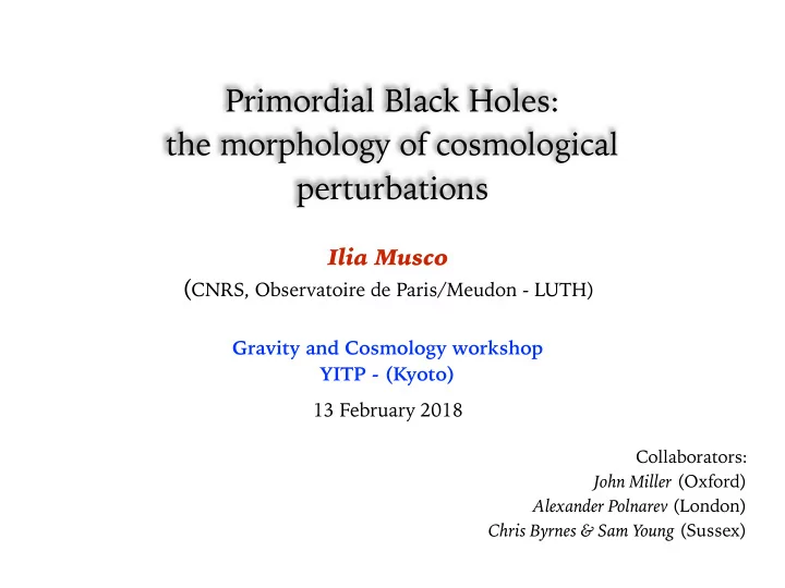
Primordial Black Holes: the morphology of cosmological perturbations Ilia Musco ( CNRS, Observatoire de Paris/Meudon - LUTH) Gravity and Cosmology workshop YITP - (Kyoto) 13 February 2018 Collaborators: John Miller (Oxford) Alexander Polnarev (London) Chris Byrnes & Sam Young (Sussex)

PBHs: A bit of history • In the early universe large amplitude perturbations of the metric can collapse into Primordial Black Holes (PBHs) [ Zeldovich & Novikov (1967); Hawking (1971)] characterized by a wide range of masses (from the Planck mass to 10 ⁶ M ⊙ for PBHs formed at the Nucleosynthesis). • Hawking evaporation effect (1974) has been inspired by the idea of PBH formation which could be small as particles and quantum effects need to taken into account. PBHs smaller than 10 15 grams would evaporate by now via Hawking evaporation, becoming possible sources of Gamma Ray Burst , Cosmic Rays , evaporation remnants as cold dark matter . • The threshold amplitude of PBH formation ( δ c ∼ c s2 ) measured at horizon crossing time Carr (1975) tell us if a perturbation collapse into a PBH or bounce and disperse into the surrounding medium. This has been confirmed by full relativistic numerical simulations Nadezin , Novikov & Polnarev (1978), Niemeyer & Jedamzik (1998, 1999); Musco et al. (2005, 2007, 2009, 2013)] suggesting that critical collapse (scaling law) might apply in the early universe, in particular during the radiation dominated era ( c s2 = 1/3 ). Harada, Nakama et al. (2013, 2014, 2015) have calculated an analytical threshold for PBH formation, proposing also a phenomenological parameterisation of PBH threshold in terms of initial density shapes.

ds 2 = − a 2 dt 2 + b 2 dr 2 + R 2 d Ω 2 ds 2 = − f 2 du 2 − 2 fb dr du + R 2 d Ω NULL TIME COSMIC TIME f du = a dt − b dr ✓ ∂ ✓ ∂ ✓ ∂ D t ≡ 1 ◆ ◆ ◆ D t ≡ 1 D r ≡ 1 D k ≡ D r + D t f ∂ u a ∂ t b ∂ r  1 ( e + p ) D k p + M Γ D t U = − R 2 + 4 π Rp + U ≡ D t R Γ ≡ D r R 1 − c 2 s ✓ D k U + 2 U Γ ◆� + c 2  � ( e + p ) D r p + M Γ s R D t U = − R 2 + 4 π Rp  D t U − D k U − 2 U Γ � D t ρ = ρ D t ρ = − ρ Γ R 2 D r ( R 2 U ) R Γ ✓ e + p ◆ D t e = e + p D t e = D t ρ D t ρ ρ ρ D t M = − 4 π R 2 pU D t M = − 4 π R 2 pU  ( Γ + U ) � a = − 4 π R ( e + p ) f D k D r a = − e + pD r p f D k M = 4 π R 2 [ e Γ − pU ] , D r M = 4 π R 2 Γ e Γ = D k R − U = 1 + U 2 − 2 M Γ 2 = 1 + U 2 − 2 M R R

Numerical Results: the method • Simulations are performed using a Lagrangian spherically symmetric GR hydro code with an adaptive grid (AMR). • We set initial conditions using a cosmic time coordinate t . • We transfer those onto a null foliation of the space time, then evolved using an observer time coordinate u . • The formation of a PBH is seen by a distant external observer (the singularity is hidden by the asymptotic formation of the apparent horizon).

Equation of State energy density: pressure: p = ( � − 1) ⇢✏ e = ⇢ (1 + ✏ ) rest mass density adiabatic index - particle degree of freedom specific internal energy (velocity dispersion) • Barotropic fluid (no rest mass density): with w ∈ [0 , 1] p = we - radiation dominated era: RADIATION ( γ = 4 / 3) w = 1 / 3 - DUST ( γ = 1) matter dominated era: w = 0 • p = K ( s ) ρ γ ( γ = 5 / 3 , 4 / 3 , 2) Polytropic fluid: - If the fluid is adiabatic (no entropy change): (constant) K ( s ) = K

Numerical Results: P BH formation/bounce IM, J. Miller - CQG (2005, 2009)

<latexit sha1_base64="pAWCRYquGQcv+zvOehkf9WUxAY=">ACQnicfVDLSgMxFM34tr6qLt0Ei1gRy7QI6kIQ3QhuFKwPOmPJZO60oZkHyR2xDv02V36BKz/AlaCIWxemtYgvPBA4OedcbnK8RAqNtn1vDQwODY+Mjo3nJianpmfys3MnOk4VhyqPZazOPKZBigiqKFDCWaKAhZ6EU6+1/VPL0FpEUfH2E7ADVkjEoHgDI1Uz587XnwFfkYPimpFXVToNl2jDgrpQ6Y6zjUgWy5+3lcCQHWKqv/JRoNGlnXq+YJfsHuhvUu6TAunjsJ6/c/yYpyFEyCXTula2E3QzplBwCZ2ck2pIG+xBtQMjVgI2s16FXToklF8GsTKnAhpT/06kbFQ63bomWTIsKl/el3xL6+WYrDpZiJKUoSIfywKUkxpt0+qS8UcJRtQxhXwryV8iZTjKNpPZczLZR/vk3qVZKWyX7aL2ws9uvY4wskEVSJGWyQXbIPjkVcLJDXkgT+TZurUerRfr9SM6YPVn5sk3WG/vJ4ewjg=</latexit> <latexit sha1_base64="pAWCRYquGQcv+zvOehkf9WUxAY=">ACQnicfVDLSgMxFM34tr6qLt0Ei1gRy7QI6kIQ3QhuFKwPOmPJZO60oZkHyR2xDv02V36BKz/AlaCIWxemtYgvPBA4OedcbnK8RAqNtn1vDQwODY+Mjo3nJianpmfys3MnOk4VhyqPZazOPKZBigiqKFDCWaKAhZ6EU6+1/VPL0FpEUfH2E7ADVkjEoHgDI1Uz587XnwFfkYPimpFXVToNl2jDgrpQ6Y6zjUgWy5+3lcCQHWKqv/JRoNGlnXq+YJfsHuhvUu6TAunjsJ6/c/yYpyFEyCXTula2E3QzplBwCZ2ck2pIG+xBtQMjVgI2s16FXToklF8GsTKnAhpT/06kbFQ63bomWTIsKl/el3xL6+WYrDpZiJKUoSIfywKUkxpt0+qS8UcJRtQxhXwryV8iZTjKNpPZczLZR/vk3qVZKWyX7aL2ws9uvY4wskEVSJGWyQXbIPjkVcLJDXkgT+TZurUerRfr9SM6YPVn5sk3WG/vJ4ewjg=</latexit> <latexit sha1_base64="pAWCRYquGQcv+zvOehkf9WUxAY=">ACQnicfVDLSgMxFM34tr6qLt0Ei1gRy7QI6kIQ3QhuFKwPOmPJZO60oZkHyR2xDv02V36BKz/AlaCIWxemtYgvPBA4OedcbnK8RAqNtn1vDQwODY+Mjo3nJianpmfys3MnOk4VhyqPZazOPKZBigiqKFDCWaKAhZ6EU6+1/VPL0FpEUfH2E7ADVkjEoHgDI1Uz587XnwFfkYPimpFXVToNl2jDgrpQ6Y6zjUgWy5+3lcCQHWKqv/JRoNGlnXq+YJfsHuhvUu6TAunjsJ6/c/yYpyFEyCXTula2E3QzplBwCZ2ck2pIG+xBtQMjVgI2s16FXToklF8GsTKnAhpT/06kbFQ63bomWTIsKl/el3xL6+WYrDpZiJKUoSIfywKUkxpt0+qS8UcJRtQxhXwryV8iZTjKNpPZczLZR/vk3qVZKWyX7aL2ws9uvY4wskEVSJGWyQXbIPjkVcLJDXkgT+TZurUerRfr9SM6YPVn5sk3WG/vJ4ewjg=</latexit> Background model & Curvature profile • The unperturbed solution, describing an expanding homogeneous universe , is given by the FRW metric: K = ±1, 0 is the curvature parameter , is the s ( t ) scale factor , and R= r circumferential radial coordinate / areal radius . s ( t ) dr 2  � ds 2 = − dt 2 + s 2 ( t ) 1 − Kr 2 + r 2 d Ω 2 • In the linear regime of cosmological perturbations, pure growing modes on the super horizon scale can be described by a time independent curvature profile ( quasi-homogeneous / gradient expansion solution ). re ζ (˜ r ) K ( r ) or ζ (˜ r ) r = ˜ K ( r ) r 2 = − ˜ r ζ 0 (˜ r ζ 0 (˜ r ) [2 + ˜ r )]

PBH formation: setting the problem • Defining the scale of the cosmological perturbations as R 0 and the cosmological horizon scale as R H := 1/H b . In the linear regime of supra horizon growing modes we can construct a small parameter (t) << 1 as: ✏ ✓ t ◆ (1+3 w ) H 2 = 8 π 3 e b ⇒ R H = 1 ✏ ( t ) := R H 3(1+ w ) ∝ H R 0 t 0 h i 1 + ✏ 2 ( t ) ˜ • Pure growing modes are given by f ( r, t ) = f 0 f ( r ) ✏ ⌧ 1 a = 1 + ✏ 2 ˜ 1 + ✏ 2 ˜ � � e = e b a e @ r R ⇣ ⌘ 1 + ✏ 2 ˜ ⇣ ⌘ 1 + ✏ 2 ˜ b = b U = HR U p 1 − K ( r ) r 2 M = 4 3 ⇡ e b R 3 ⇣ ⌘ 1 + ✏ 2 ˜ 1 + ✏ 2 ˜ ⇣ ⌘ M R = s ( t ) r R • In the linear regime , when << 1, the curvature profile is time independent ✏ because pressure gradients are negligible, and can be used as the only independent source of perturbations.