The Distribution of The Total Dividend Payments in a MAP Risk Model - PowerPoint PPT Presentation

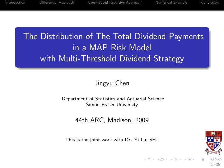
Introduction Differential Approach Layer-Based Recursive Approach Numerical Example Conclusion The Distribution of The Total Dividend Payments in a MAP Risk Model with Multi-Threshold Dividend Strategy Jingyu Chen Department of Statistics and Actuarial Science Simon Fraser University 44th ARC, Madison, 2009 This is the joint work with Dr. Yi Lu, SFU 1 / 25

Introduction Differential Approach Layer-Based Recursive Approach Numerical Example Conclusion Outline of Topics Introduction 1 Differential Approach 2 Layer-Based Recursive Approach 3 Numerical Example 4 Conclusion 5 2 / 25

Introduction Differential Approach Layer-Based Recursive Approach Numerical Example Conclusion Sample Surplus Process Surplus U(t) premiums claims premium rate = c u ruin 0 Time t 3 / 25

Introduction Differential Approach Layer-Based Recursive Approach Numerical Example Conclusion The Classical Risk Model The surplus process { U ( t ); t ≥ 0 } with U (0) = u , s.t. dU ( t ) = cdt − dS ( t ) , t ≥ 0 . Premiums are collected continuously at a constant rate c A sequence of non-negative claim amounts r.v. { X n ; n ∈ N + } Number of claims up to time t , N ( t ) ∼ Poisson( λ t ) Aggregate claim amounts up to time t , S ( t ) = � N ( t ) n =1 X n Time of ruin τ = inf { t ≥ 0 : U ( t ) < 0 } 4 / 25

Introduction Differential Approach Layer-Based Recursive Approach Numerical Example Conclusion MAP Risk Model MAP ( � α, D 0 , D 1 ) Initial distribution, � α Intensity matrix, D 0 + D 1 Intensity of state changing without claim, D 0 ( i , j ) ≥ 0, j � = i Intensity of state changing with claim, D 1 ( i , j ) ≥ 0 The diagonal elements of D 0 are negative values, s.t. D 0 + D 1 = 0 Special cases: classical risk model, Sparre-Andersen risk model, Markov-modulated risk model Reference: Badescu et al. (2007), Badescu (2008), Ren (2009), 5 / 25

Introduction Differential Approach Layer-Based Recursive Approach Numerical Example Conclusion Various Dividend Strategies Surplus premiums claims b u ruin 0 Time t 6 / 25

Introduction Differential Approach Layer-Based Recursive Approach Numerical Example Conclusion Various Dividend Strategies Surplus premiums claims b u ruin 0 Time t 7 / 25

Introduction Differential Approach Layer-Based Recursive Approach Numerical Example Conclusion Various Dividend Strategies Surplus premiums claims b 2 b 1 u ruin 0 Time t 8 / 25

Introduction Differential Approach Layer-Based Recursive Approach Numerical Example Conclusion Multi-Threshold MAP Risk Model Thresholds: 0 = b 0 < b 1 < · · · < b n < b n +1 = ∞ Premium rate c k for b k − 1 ≤ u < b k , k = 1 , · · · , n + 1 c = c 1 > c 2 > · · · > c n > c n +1 ≥ 0 Time of ruin τ B = inf { t ≥ 0 : U B ( t ) < 0 } Surplus process { U B ( t ); t ≥ 0 } satisfies dU B ( t ) = c k dt − dS ( t ) , b k − 1 ≤ U B ( t ) < b k Claim amounts distribution f i , j , F i , j and Laplace transformation ˆ f i , j ( s ) 9 / 25

Introduction Differential Approach Layer-Based Recursive Approach Numerical Example Conclusion Expected Discounted Dividend Payments D ( t ) is the aggregate dividends paid by time t Define � τ B e − δ t dD ( t ) , D u , B = u ≥ 0 , 0 to be the present value of dividend payments prior to ruin, given the initial surplus u Define V i ( u ; B ) = E i [ D u , B | U B (0) = u ] , i ∈ E , to be the expected present value of dividend payments prior to ruin, given the initial surplus u and the initial phase i ∈ E 10 / 25

Introduction Differential Approach Layer-Based Recursive Approach Numerical Example Conclusion Expected Discounted Dividend Payments The piecewise vector function of the expected present value of the total dividend payments prior to ruin �  V 1 ( u ; B ) 0 ≤ u < b 1 ,   � � V ( u ; B ) = V k ( u ; B ) b k − 1 ≤ u < b k , k = 2 , · · · , n , �  V n +1 ( u ; B ) b n ≤ u < ∞ .  � V k ( u ; B ) = ( V 1 , k ( u ; B ) , · · · , V m , k ( u ; B )) ⊤ for b k − 1 ≤ u < b k and k = 1 , · · · , n + 1 11 / 25

Introduction Differential Approach Layer-Based Recursive Approach Numerical Example Conclusion Differential Approach Typical approach in various risk models Integro-differential equations are involved Can be derived and solved analytically for some families of claim amounts distribution Mainly in Gerber-Shiu discounted penalty function Techniques can be applied to the dividend payments problems Lin and Sendova (2008), classical risk model Lu and Li (2009), Sparre Andersen risk model 12 / 25

Introduction Differential Approach Layer-Based Recursive Approach Numerical Example Conclusion Integro-Differential Equation for � V k ( u ; B ) Condition on the events occurring in a small time interval [0 , h ] No change in the MAP state A change in the MAP state accompanied by no claim arrival A change in the MAP state accompanied by a claim arrival; Claim amounts may vary Two or more events occur 13 / 25

Introduction Differential Approach Layer-Based Recursive Approach Numerical Example Conclusion Integro-Differential Equation for � V k ( u ; B ) Integro-differential equation, for b k − 1 ≤ u < b k � u − b k − 1 c k � k ( u ; B ) = δ� V k ( u ; B ) − D 0 � Λ f ( x ) � V ′ V k ( u ; B ) − V k ( u − x ; B ) dx − � γ k ( u ) 0 � u − b l − 1 where γ i , k ( u ) = ( c − c k ) + � m j =1 D 1 ( i , j ) � k − 1 V j , l ( u − x ; B ) dF i , j ( x ) l =1 u − b l Solution � u − b k − 1 V k ( b k − 1 ; B ) − 1 V k ( u ; B ) = v k ( u − b k − 1 ) � � v k ( t ) � γ k ( u − t ) dt c k 0 ��� � − 1 � � where v k ( u − b k − 1 ) = L − 1 s − δ I + 1 c k ( D 0 + Λ ˆ f ( s )) c k 14 / 25

Introduction Differential Approach Layer-Based Recursive Approach Numerical Example Conclusion Recursive Expression for � V k ( u ; B ) Define vector function � V k ( u ) for u ≥ b k − 1 � u − b k − 1 V k ( b k − 1 ) − 1 V k ( u ) = v k ( u − b k − 1 ) � � v k ( t ) � γ k ( u − t ) dt c k 0 Restrict to b k − 1 ≤ u < b k , compare with � V k ( u ; B ) V k ( u ; B ) = � � V k ( u ) + v k ( u − b k − 1 ) � π k ( B ) , b k − 1 ≤ u < b k Continuity condition at b k − 1 , k = 1 , · · · , n π k +1 ( B ) = � V k ( b k ) − � � V k +1 ( b k ) + v k ( b k − b k − 1 ) � π k ( B ) Final boundary condition when k = n + 1 π n +1 ( B ) = � V n ( b n ) − � π n ( B ) = � � V n +1 ( b n ) + v n ( b n − b n − 1 ) � 0 15 / 25

Introduction Differential Approach Layer-Based Recursive Approach Numerical Example Conclusion Layer-Based Recursive Algorithm Computational disadvantage of the recursive algorithm based on integro-differential equations Constant vectors can only be solved in the last layer Infeasible to compute for large number of layers Layer-based approach Condition on the exit times of the surplus out of each layer Calculate successively for increasing number of layers � The ( k − 1)-layer model The k -layer model ⇐ Classical one-layer model Reference: Albrecher and Hartinger (2007) 16 / 25

Introduction Differential Approach Layer-Based Recursive Approach Numerical Example Conclusion Sample Path of One-Layer Model with Dividend Payments Surplus U 1,k (t) premiums claims u 0 Time t 17 / 25

Introduction Differential Approach Layer-Based Recursive Approach Numerical Example Conclusion Time Value of Upper Exit Define τ ∗ ( u , a , b ) = inf { t ≥ 0 : U ( t ) / ∈ [ a , b ] | U (0) = u } Define � τ ∗ ( u , a , b ) if U ( τ ∗ ( u , a , b )) = b τ + ( u , a , b ) = ∞ if U ( τ ∗ ( u , a , b )) < a and � if U ( τ ∗ ( u , a , b )) = b ∞ τ − ( u , a , b ) = τ ∗ ( u , a , b ) if U ( τ ∗ ( u , a , b )) < a Laplace transform of τ + k ( u , 0 , b ) � e − δτ + � k ( u , 0 , b ) 1 [ J ( τ + � B i , j , k ( u , b ) = E � J (0) = i k ( u , 0 , b ))= j ] given initial phase i and reaching b in phase j Reference: Gerber and Shiu (1998), Albrecher and Hartinger (2007) 18 / 25

Introduction Differential Approach Layer-Based Recursive Approach Numerical Example Conclusion Time Value of Upper Exit For δ > 0 and k ∈ N + , we have 1 = if u ≥ b B k 1 , B k = 0 , if u < 0 For 0 ≤ u < b k − 1 2 � B k − 1 ( u , b ) , if b ≤ b k − 1 B k ( u , b ) = B k − 1 ( u , b k − 1 ) B k ( b k − 1 , b ) , if b ≥ b k − 1 For b k − 1 ≤ u ≤ b 3 B k ( u , b ) = B 1 , k ( u − b k − 1 , b − b k − 1 ) + M k ( u − b k − 1 ) − B 1 , k ( u − b k − 1 , b − b k − 1 ) M k ( b − b k − 1 ) Parallel results in matrix form Reference: Albrecher and Hartinger (2007) 19 / 25

Introduction Differential Approach Layer-Based Recursive Approach Numerical Example Conclusion Sample Path for 0 ≤ u ≤ b k − 1 Surplus U B (t) premiums claims b k-1 u ruin 0 Time t 20 / 25

Introduction Differential Approach Layer-Based Recursive Approach Numerical Example Conclusion Sample Path for u ≥ b k − 1 Surplus U B (t) premiums claims u b k-1 0 Time t 21 / 25