The Dawning of the Age of Stochasticity For over two millennia, - PowerPoint PPT Presentation
The Dawning of the Age of Stochasticity For over two millennia, Aristotles logic has ruled over the thinking of western intellectuals. All precise theories, all sci- entific models, even models of the process of thinking itself, have in
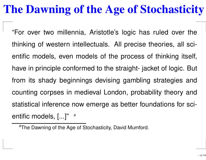
The Dawning of the Age of Stochasticity “For over two millennia, Aristotle’s logic has ruled over the thinking of western intellectuals. All precise theories, all sci- entific models, even models of the process of thinking itself, have in principle conformed to the straight- jacket of logic. But from its shady beginnings devising gambling strategies and counting corpses in medieval London, probability theory and statistical inference now emerge as better foundations for sci- entific models, [...]” a a The Dawning of the Age of Stochasticity, David Mumford. . – p.1/34
Why do we need probabilities? a To deal with the complexity of the reality i.e. study emerging statistical behavior of overwhelmingly large and complex systems e.g. a cubic centimeter of solid matter contains about 10 24 atoms, but we still have good statistical models of the (somewhat surprising) behavior of melting ice frequentist ’s realm To represent beliefs about this reality bayesian ’s realm a You don’t have to read the footnotes to follow . – p.2/34
Basic building blocks (1/3) First: A probability space (Ω , F , P ) Ω is a set and can be interpreted as the collections of all possible “states” ω ∈ Ω that the system can take We will call a subset A ⊆ Ω an event . A sigma-field F , the set of all possible events. We will a not worry about this guy for today. P : F → [0 , 1] is a probability measure , it gives probabilities to events. Axiomatic properties: P (Ω) = 1 � ∞ i =0 P ( A i ) = P ( � ∞ i =0 A i ) for all disjoint A i ’s a See for instance G.B. Folland: Real Analysis. . – p.3/34
Basic building blocks (2/3) Second: Random variables (r.v.) X, Y, ... Can be interpreted as “measurements” on the system a Formally a map from the probability space to the reals This is the object of interest for the statistician Notation: for R ⊆ R , ( X ∈ R ) := X − 1 ( R ) = { ω ∈ Ω : X ( ω ) ∈ R } , same with = , ≤ , ≥ , <, > instead of ∈ The distribution of a r.v. X : for R ∈ R , P X ( R ) = P ( X ∈ R ) . Note that this is a probability measure on the real line. a Actually, this can be generalized, for instance to euclidean spaces, topological spaces, or measurable spaces (preferred by modern treatments to facilitate com- positions). Euclidean spaces will suffice for today. . – p.4/34
Basic building blocks (3/3) Third: Expectations E Enables us to make “statements” on a r.v., by averaging out its values For a r.v. that takes finitely many values { x 0 , . . . , x n } (a simple r.v.): EX := � n i =0 x i P ( X = x i ) = � n i =0 x i p X ( x i ) a This def. can be generalized to arbitrary r.v. a Using Lebesgue integration. The basic idea is the same as the Riemann in- tegral (limit of finite approximations), but the Lebesgue integral partition the image rather than the domain to perform approximation. This leads to a nicer theory— better interaction b/w limits and integrals. . – p.5/34
Properties of expectation It is very important to know how to manipulate expectations: Expectations are linear operators on the space of r.v.: E [ aX + Y ] = aEX + EY They are monotone: X ≤ Y implies that EX ≤ EY . a (Jensen’s inequality) log EX ≥ E log X a whenever E | X | < ∞ (in which case we say X ∈ L 1 ( P ) ), log could be replaced by any concave function. . – p.6/34
Important notations and trick Cumulative Distribution Function (CDF): F X ( x ) = P ( X ≤ x ) Densities : used for concrete representation of continuous distributions. A function f : R → [0 , ∞ ) is the density of a probability measure Q on the real line if a Note � Q ( R ) = R f ( x ) dx for all event R on the real line. that single-point probabilities do not characterize continuous distribution (they are all 0). If g : R → R , g ( X ) a r.v., P X has density f , then � Eg ( X ) = g ( x ) f ( x ) dx a Again, this can be made more abstract. In general, the existence of a density is characterized by the Radon-Nikodym theorem . – p.7/34
Examples: Binomial Distribution a N , bias of the Parameters: number of coin tosses coin p Let X be the number of heads out of N coin tosses, with coins not necessarily fair (probability p of a head, q of a tail p n q N − n for n ∈ { 0 , . . . , N } � N � p ( n ) = n a the generalization to dices is called a Multinomial Distribution, n 1 ! ...n k ! p n 1 . . . p n 2 , for integers � n i = N N ! p ( n 1 , . . . , n k ) = . – p.8/34
Examples: Uniform Distribution Parameters: a nonempty interval ( a, b ) The probability that X falls inside a subinterval is proportional to its length, and invariant for translation [ x ∈ ( a, b )] 1 Density: f ( x ) = � b − a . – p.9/34
Examples: Normal Distribution Two parameters, the mean µ , and the variance, σ 2 � ( x − µ ) 2 1 � Density: f ( x ) = 2 πσ 2 exp √ 2 σ 2 We will come back on the reasons of its importance . – p.10/34
Many others B( α,β ) x α − 1 (1 − x ) β − 1 1 Beta, f ( x ; α, β ) = 1 B( α,β ) x α − 1 (1 − x ) β − 1 Gamma, f ( x ; α, β ) = � K 1 i =1 x α i − 1 Dirichlet, f ( x ; α ) = B( α ) i They will be useful for statistical Bayesian inference. . – p.11/34
Conditioning to represent belief P ( A | B ) = P ( A ∩ B ) , whenever P ( B ) > 0 B The probability that event A occurs given that we observed event B Important properties and definitions: Chain rule: P ( X = x, Y = y ) = P ( X = x ) P ( Y = y | X = x ) a conditional expectation: Discrete E [ X | A ] = � i x i P ( X = x i | A ) a Developing formally the general theory of conditional probability and expecta- tion is more involved: see Probability and Measure, P . Billingsley . – p.12/34
Statistical independence Independence: X, Y are statistically independent if F X,Y ( x, y ) = F X ( x ) F X ( y ) for all x, y ∈ R When X, Y have densities, this is true iff f X,Y ( x, y ) = f X ( x ) f Y ( y ) Crucial for statistical independence If there is no independence between the r.v. under study, we cannot do anything! If there are too few, there is a risk of oversimplification a is a very useful way to define Graphical models distributions on r.v. that have a good trade-off b/w complexity of inference and expressivity of the model a See http://www.cs.ubc.ca/ murphyk/Bayes/bnintro.html for a quick tutorial. . – p.13/34
Bayes Theorem The foundation of Baysian inference P ( A | B ) = P ( B | A ) P ( A ) whenever P ( B ) > 0 P ( B ) P ( A ) is the prior probability . It is “prior” in the sense that it does not take into account any information about B . P ( A | B ) is also called the posterior probability because it is derived from or depends upon the specified value of B . P ( B ) is marginal probability of B , and acts as a normalizing constant . – p.14/34
How to evaluate expectations in practice In practice it is hard to compute expectations exactly Example: To check if a coin is fair, you flip it 100 times and check if the number of head is approximately 50. The Law of Large Numbers: for Independent and Identically Distributed (iid) r.v. X 1 , X 2 , . . . , � n lim n →∞ 1 a i =1 X i = EX n Justification for frequentist’s approach Monte Carlo integration more and more used to approximate integrals, even outside statistics a almost everywhere, provided that the r.v.’s are L 1 . – p.15/34
The Central Limit Theorem (CLT) This is a statement in the limit... we only have finitely many samples in practice Observe that � n i =1 X i is a r.v. as well If we can compute its distribution, we can say how “sharply peaked” it is, and give confidence intervals on our MC estimate Problem: this distribution is typically very hard to compute! (Note: if X i has density f X i and Y = X 1 + X 2 , a ) it DOES NOT imply that Y has density f X 1 + f X 2 a A convolution would have to be computed. . – p.16/34
The Central Limit Theorem (CLT) Solution: the CLT tell us that this distribution converges to a normal So this is still a limit statement, but in practice, convergence of CLT is usually very fast (20 samples already gives a good approximation in many cases) Solution: the CLT tell us that this distribution converges to a normal So this is still a limit statement, but in practice, convergence of CLT is usually very fast (20 samples already gives a good approximation in many cases) This also a motivation for using Normal Distribution in some systems . – p.17/34
Basic Setup of Statistics Again, let us start with Frequentist statistics We are given a statistic T ( X 1 , . . . , X n ) , i.e. a random variable that depends on the data that represents an estimator for some unknown quantity θ buried in the system. Examples: we want to determine is a coin is fair (here we can estimate a real number, the probability that we get a head) we want to learn to discriminate between normal traffic and DoS (here we want to estimate a much more complex object, a decision function ) We want to evaluate how good the estimator is . – p.18/34
Criteria Bias: ET ( X 1 , . . . , X n ) − θ Variance: V ar ( T ) = E ( T − ET ) 2 Property: V ar [ aT + b ] = a 2 V arT Property: If T 1 , T 2 independent, V ar [ T 1 + T 2 ] = V ar [ T 1 ] + V ar [ T 2 ] There is a trade-off between bias and variance Robustness to outliers . – p.19/34
Recommend
More recommend
Explore More Topics
Stay informed with curated content and fresh updates.
