TESTING AND CORRECTING FOR ENDOGENEITY IN NONLINEAR UNOBSERVED - - PowerPoint PPT Presentation

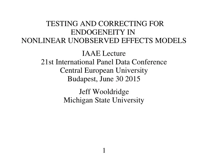
TESTING AND CORRECTING FOR ENDOGENEITY IN NONLINEAR UNOBSERVED EFFECTS MODELS IAAE Lecture 21st International Panel Data Conference Central European University Budapest, June 30 2015 Jeff Wooldridge Michigan State University

1

• 1. Introduction
• 2. Linear Model
• 3. Exponential Model
• 4. Probit Response Function
• 5. Empirical Example
• 6. Extensions and Future Directions

2

• 1. Introduction

∙ In unobserved effects models we can think of two kinds of

endogeneity for an explanatory variable:

• 1. Correlation with unobserved effect(s) (time constant)
• 2. Correlation with innovations (time varying)

3

∙ Application to linear model: Levitt (1996, QJE), effects of

prison size on violent crime.

∙ Nonlinear models: Can combine the correlated random

effects (CRE) and control function (CF) approaches for certain nonlinear models. 4

∙ Papke and Wooldridge (2008, J of E) provides one

• approach. Simple but not ideal for testing purposes: It

conflates the two kinds of endogeneity.

∙ Application to effects of spending on school/district test

pass rates.

∙ Here focus on continuous endogenous explanatory

variables (EEVs), but some suggestions for discrete EEVs. 5

∙ Other Approaches:

• 1. “Fixed Effects” (Heterogeneity as parameters to

estimate):  Incidental parameters problem with small T.  Bias adjustments available for parameters and average partial effects, but usually stationarity and weak dependence (even independence) are assumed.  Difficult to incorporate time effects.  Endogenous explanatory variables? 6

• 2. Conditional MLE:

 Only works in special cases.  Relies on conditional independence across time.  Partial effects in nonlinear models often unidentified.  Exentensions to EEVs?

• 3. Finite Number of Types (Bonhomme and Manresa)

 Conditional Independence  Nonlinear Models?  Extension to EEVs? 7

Ideal FE CMLE CRE Restricts Dci|xi? No No No Yes Incidental Parameters with Small T? No Yes No No Restricts Time Series Dependence/Heterogeneity? No Yes1 Yes2 No Restricts Amount of Heterogeneity? No No3 Yes No APEs Identified? Yes Yes4 No Yes Unbalanced Panels? Yes Yes Yes Yes5 Can Estimate Dci? Yes Yes4 No Yes6 Endogenous Explanatory Variables? Yes Yes4 No7 Yes

8

• 1. The large T approximations assume weak dependence and often stationarity.
• 2. Usually conditional independence, unless estimator is inherently fully robust (linear, Poisson).
• 3. Need at least one more time period than sources of heterogeneity.
• 4. Subject to the incidental parameters problem.
• 5. Subject to exchangeability restrictions.
• 6. Under conditional independence or some other restriction.
• 7. Unless one makes parametric assumptions on the reduced form and imposes conditional

independence.

9

• 2. Linear Model

∙ Consider a “structural” equation

yit1  xit11  ci1  uit1 where xit1  zit1,yit2

∙ The outside instruments are zit2. ∙ zit1 can include time effects, but supress.

10

∙ Both zit and yit2 may be correlated with ci1. ∙ Assume zit is strictly exogenous with respect to uit1:

Covzit,uir1  0, all t,r  1,...,T

∙ yit2 may be correlated with uit1 (across all time

periods).

∙ Given a rank condition, 1 can be estimated by fixed

effects IV (FEIV). 11

∙ How can we test the null hypothesis that yit2 is

exogenous with respect to uit1?

∙ Hausman test comparing FE and FEIV.

 Cumbersome due to deficient rank.  Original Hausman test not robust to serial correlation

• r heteroskedasticity in uit1.

12

∙ Variable Addition Test (Control Function):

• 1. Estimate the reduced form of yit2,

yit2  zit2  ci2  uit2, by fixed effects, and obtain the FE residuals,  üit2  ÿit2 − z ̈ it ̂ 2 ÿit2  yit2 − T−1 ∑

r1 T

yir2 13

• 2. Estimate the equation

yit1  xit11   üit21  ci1  errorit1 by usual FE and compute a robust test of H0 : 1  0.

∙ In step (2), 

̂

1 is the FEIV estimator.

∙ Note that the nature of yit2 is unrestricted (discrete,

continuous, both features). 14

∙ We can also use a correlated random effects approach, but

some but some care is needed to get a proper test.

∙ The Mundlak equation for yit2 is

yit2  2  zit2  z ̄ i2  ai2  uit2 z ̄ i  T−1 ∑

t1 T

zit

∙ We are operating as if

Covzit,uis2  0, all t,s Covzit,ai2  0, all t 15

∙ Key: How should we apply the Mundlak device to ci1 in

yit1  xit11  ci1  uit1?

∙ Projecting ci1 only onto z

̄ i is fine for estimation.

∙ For testing, it does not distinguish between

Covyit2,ci1 ≠ 0 and Covyit2,uis1 ≠ 0. 16

∙ Better is to project ci1 onto z

̄ i,v ̄ i2 where yit2  2  zit2  z ̄ i2  vit2 ci1  1  z ̄ i1  v ̄ i21  ai1 Covzi,ai1  0 Covyi2,ai1  0 17

∙ Plugging in gives the estimating equation

yit1  xit11  1  z ̄ i1  v ̄ i21  ai1  uit1  xit11  1  z ̄ i1  y ̄ i21  ai1  uit1

∙ By the Mundlak device, ai1 is uncorrelated with all RHS

• bservables.

∙ By assumption, zi is uncorrelated with uit1. ∙ Now test whether yit2, equivalently vit2, is uncorrelated

with uit1. 18

• 1. Run a pooled OLS regression (or use random effects),

yit2  2  zit2  z ̄ i2  vit2, and obtain the residuals, v ̂ it2.

• 2. Estimate

yit1  xit11  1  z ̄ i1  y ̄ i21  v ̂ it21  errorit1 by POLS or RE.

• 3. Use a robust Wald test of H0 : 1  0.

19

∙ Algebra:

(i)  ̂

1 in step (2) is the FEIV estimator.

(ii)  ̂ 1 is identical to that from estimating yit1  xit11   üit21  ci1  errorit1 by FE.

∙ Result (i) still holds if y

̄ i2 is dropped from the estimating equation, but (ii) does not. 20

∙ Conclusion: In using the CRE/CF approach for testing

H0 : Covyit2,uis1  0, use the equations yit2   ̂ 2  zit ̂ 2  z ̄ i ̂ 2  v ̂ it2 yit1  xit11  1  z ̄ i1  y ̄ i21  v ̂ it21  errorit1

∙ Also works in the unbalanced case when the complete

cases are used (Joshi and Wooldridge, 2015). 21

∙ What about using Chamberlain in place of Mundlak? ∙ Reusing notation, with

zi  zi1,...,ziT, yi2  yi12,...,yiT2, yit2   ̂ 2  zit ̂ 2  zi ̂ 2  v ̂ it2 yit1  xit11  1  zi1  yi21  v ̂ it21  errorit1

∙ Estimates of 1 and 1 are are identical to Mundlak, as is

robust Wald test. (POLS or RE). 22

∙ Conclusion: Include time averages of zit and yit2 to

• btain a clean test of endogeneity of yit2 with respect to

uit1.

∙ If POLS or RE are used, Chamberlain  Mundlak. ∙ All goes through with time effects. ∙ Time constant variables can be included in the CRE/CF

approach. 23

∙ Ignoring the pre-testing problem, a strategy for testing is:

• 1. If the VAT rejects, use FEIV.

 Or, then test REIV against FEIV, as instruments may be “super” exogenous.

• 2. If the VAT fails to reject, use FE or compare RE and FE.

24

• 3. Exponential Model

∙ Fully robust test for exogeneity:

• 1. Estimate the reduced form for yit2 by fixed effects and
• btain the FE residuals,

 üit2  ÿit2 − z ̈ it ̂ 2

• 2. Use FE Poisson on the mean function

“Eyit1|zit1,yit2, üit2,ci1  ci1 expxit11   üit21” and use a robust Wald test of H0 : 1  0. 25

∙ The null hypothesis is

H0 : Eyit1|zi1,yi2,üit2,ci1  Eyit1|zit1,yit2,ci1  ci1 expxit11

∙ Algebra: The Poisson FE estimates of 1,1 are

unchanged if we estimate the Mundlak reduced form: yit2  2  zit2  z ̄ i2  vit2 and use residuals, v ̂ it2 (v ̂ it2 ≠  üit2 but  v ̈ it2   üit2). 26

∙ For testing, no restrictions are put on the RF of yit2. ∙ When would the Mundlak/FE Poisson approach be

consistent for 1?

∙ Assume that

Eyit1|zi,yi2,ci1,uit1  Eyit1|zit1,yit2,ci1,uit1  ci1 expxit11  uit1 where xit1 can be any function of zit1,yit2. 27

∙ The reduced form is

yit2  2  zit2  z ̄ i2  ai2  uit2 vit2  ai2  uit2

∙ Sufficient is

uit1  uit21  eit1  vit21 − ai21  eit1 eit1  zi,ci1,ci2,ui2 28

∙ This appears to impose a restriction of only

contemporaneous correlation between uit1 and uit2. How important is it?

∙ In the linear case it makes no difference.

29

∙ Is consistently estimating 1 enough? ∙ The average structural function (Blundell and Powell,

2003) is identified: ASFxt1  Eci1,uit1ci1 expxt11  uit1  Eci1,uit1ci1 expuit1expxt11

∙ But the average partial effects are not generally identified. ∙ For a continuous xt1j,

APEtj  1jExit1,ci1,uit1ci1 expxit11  uit1 30

∙ A CRE/CF approach identifies both. What could it look

like?

∙ At least two choices. Let

Eyit1|zit1,yit2,ci1,uit1  ci1 expxit11  uit1 vit1  ci1 expuit1 yit2  2  zit2  z ̄ i2  vit2

• 1. Use Mundlak (or Chamberlain) on

Dvit1|zi,vit2  Dvit1|z ̄ i,vit2 (Papke and Wooldridge, 2008). 31

∙ Uses weaker exogeneity requirements (but not in linear

model).

∙ Cannot use GLS-type methods; pooled methods or GMM

from moment conditions.

∙ Does not lead to cleanest test of endogeneity.

32

• 2. Use Mundlak (or Chamberlain) on

Dvit1|zi,vi2  Dvit1|z ̄ i,v ̄ i2,vit2  Dvit1|z ̄ i,y ̄ i2,vit2

∙ Strict exogeneity is assumed, so GLS-type procedures can

be used.

∙ Separates endogeneity of yit2 with respect to ci1 and

uit1.

∙ Because of the linear index structure, we can use the

Mundlak residuals or FE residuals for the RF of yit2. 33

∙ In the simplest case, the estimating equation is

Eyit1|zi,yi2  exp1  xit11  z ̄ i1  y ̄ i21  vit21 and the Mundlak or FE residuals are plugged in for vit2.

∙ One can apply GLS (“generalized estimating equations)

methods, or GMM.

∙ Unlike in the linear case, no equivalance between CRE and

FE Poisson estimates.

∙ Wooldridge (1991)/Windmeijer (2000) moments approach

is an alternative. 34

• 4. Probit Response Function

∙ Now consider a probit conditional mean for yit1 ∈ 0,1:

Eyit1|zi,yi2,rit1  Eyit1|zit1,yit2,rit1  xit11  rit1

∙ Thinking of

rit1  ci1  uit1

∙ For continuous EEVs,

yit2  2  zit2  z ̄ i2  vit2 35

∙ Assume

vit2 is independent of zi.

∙ Key assumption:

Drit1|zi,vi2  Drit1|z ̄ i,v ̄ i2,vit2  Drit1|z ̄ i,y ̄ i2,vit2

∙ Leading case: homoskedastic normal with linear mean:

rit1|z ̄ i,y ̄ i2,vit2  Normal1  z ̄ i1  y ̄ i21  vit21,1 (Variance normalization has no effect on ASF or APEs.) 36

∙ Then

Eyit1|zi,yi2  xit11  1  z ̄ i1  y ̄ i21  vit21 and two-step procedures are immediate:

• 1. Obtain v

̂ it2 by pooled OLS.

• 2. Insert v

̂ it2 in place of vit2, use pooled (fractional) probit.

∙ Can use a quasi-GLS procedure (GEE) because of strict

exogeneity.

∙ Can test H0 : 1  0 using a robust Wald test.

37

∙ ASF is identified from

ASFxt1  Ez

̄ i,y ̄ i2,vit2xt11  1  z

̄ i1  y ̄ i21  vit21 ASFxt1  N−1 ∑

t1 T

xt1 ̂

1  

̂ 1  z ̄ i ̂

1  y

̄ i2 ̂ 1  v ̂ it2 ̂ 1

∙ APEs:

1jExit1,z

̄ i,y ̄ i2,vit2xit11  1  z

̄ i1  y ̄ i21  vit21

∙ Stata margins command gets the correct estimates, but

does not adjust inference for two-step estimation. 38

∙ Lots of useful embellishments. For example,

Varrit1|z ̄ i,y ̄ i2,vit2  exp2z ̄ i1  y ̄ i21  vit21

∙ Run a heteroskedastic “probit” with mean function

depending on 1,xit1,z ̄ i,y ̄ i2,v ̂ it2 and variance function depending on z ̄ i,y ̄ i2,v ̂ it2. 39

∙ The ASF is consistently estimated as

ASFxt1  N−1 ∑

t1 T

 xt1 ̂

1  

̂ 1  z ̄ i ̂

1  y

̄ i2 ̂ 1  v ̂ it2 ̂ 1 exp z ̄ i ̂ 1  y ̄ i2 ̂ 1  v ̂ it2 ̂ 1

∙ Stata 14 does the estimation with fracreg (pooled

estimation).

∙ Stata margins (should) give the correct estimates for the

APEs because xit1 appears only in the “mean” function. 40

∙ In the spirit of Blundell and Powell (2004, REStud), one

can directly use flexible functional forms (squares, interactions, higher order terms) in xit1,z ̄ i,y ̄ i2,v ̂ it2 and compute partial effects with respect to xit1. Average out the other variables.

∙ As in Altonji and Matzkin (2005, Econometrica), functions

• ther than time averages can be used. Can use

nonexchangeable functions, too. 41

• 5. Empirical Example

∙ Papke and Wooldridge (2008), Michigan School Reform. ∙ math4, a pass rate, is a fractional response. ∙ “Foundation Allowance” as an IV for average district

spending.

∙ Other controls: enrollment, poverty rate, year effects. ∙ Uses a kinked relationship. IV is strong. ∙ N  501, T  7

42

Model: Linear Linear FProbit FProbit Estimation: FE FEIV PQMLE PQMLE Coef Coef Coef APE Coef APE lavgrexp .377 .420 .821 .277 .797 .269 (.071) (.115) (.334) (.112) (.338) (.114) v ̂ 2 — −.060 .076 −.666 — (.146) (.145) (.396) lavgrexp? — — Yes No 43

• 6. Extensions and Future Directions

∙ Extension to discrete EEVs. Lose identification without

strong assumptions.  Can combine CRE and use one-step pooled quasi-MLE (“bivariate probit” is an example, as in Wooldridge (2014, J

• f E).

 Use generalized residuals as the CFs, such as grit2  yit2wit ̂ 2 − 1 − yit2−wit ̂ 2 when yit2 follows a reduced form probit. 44

∙ Unbalanced panels. Condition on time averages and

number of time periods and use complete cases (in reduced forms and CREs).

∙ Dynamic models with heterogeneity and EEVs (Giles and

Murtazashvili, 2013, JEM).

∙ Resiliency to model misspecification? (CRE functions,

control functions, and semiparametrics.) 45